

Tag: Fed
Confluence of Ideas – #34 “The 2024 Outlook: Slow-Bicycle Economy” (Posted 12/18/23)
Asset Allocation Bi-Weekly – #94 “Have Policymakers Solved the Tinbergen Problem?” (Posted 3/27/23)
Asset Allocation Bi-Weekly – #92 “Federal Reserve Policymakers in 2023: Hawks or Doves?” (Posted 2/27/23)
Asset Allocation Bi-Weekly – #84 “The Federal Reserve’s Big Policy Mistake” (Posted 9/19/22)
Bi-Weekly Geopolitical Podcast – #12 “The 2022 Mid-Year Geopolitical Outlook” (Posted 6/21/22)
Bi-Weekly Geopolitical Report – The 2022 Mid-Year Geopolitical Outlook (June 21, 2022)
by Bill O’Grady and Patrick Fearon-Hernandez, CFA | PDF
(N.B. Due to the Fourth of July holiday, our next geopolitical report will be published on July 18.)
As is our custom, we update our geopolitical outlook for the remainder of the year as the first half comes to a close. This report is less a series of predictions as it is a list of potential geopolitical issues that we believe will dominate the international landscape for the rest of the year. It is not designed to be exhaustive; instead, it focuses on the “big picture” conditions that we believe will affect policy and markets going forward. They are listed in order of importance.
Issue #1: The Russia-Ukraine War
Issue #2: Xi as China’s President for Life
Issue #3: The Global Food Crisis
Issue #4: Weather Disruptions
Issue #5: Latin American Politics
Issue #6: The U.S. Midterms
Issue #7: Fed Policy and the Dollar
Quick Hits: This section is a roundup of geopolitical issues we are watching that haven’t risen to the level of the concerns described above but should be monitored.
Don’t miss the accompanying Geopolitical Podcast, available on our website and most podcast platforms: Apple | Spotify | Google
Asset Allocation Bi-Weekly – #76 “The Problem of Financial Conditions” (Posted 5/31/22)
Asset Allocation Bi-Weekly – The Problem of Financial Conditions (May 31, 2022)
by the Asset Allocation Committee | PDF
Among the financial pundit class, there has been a growing call to weaken financial conditions. What are financial conditions? They include credit spreads, the level of interest rates, the level of equities, the level of market volatility, the dollar’s exchange rate, etc. Weaker financial conditions mean that borrowing costs rise, and the perceived risk of investment increases. By increasing the costs of investment and borrowing, market participants (households, firms, etc.) will often exert greater caution, and this practice will tend to slow growth in the economy. Essentially, the argument is that with inflation running “hot,” using weaker financial conditions to slow investment and consumption will eventually lead to less inflation.
However, managing financial conditions isn’t a straightforward process. Once financial conditions begin to deteriorate, they can almost take on “lives of their own.” In a sense, financial panics are evidence of rapidly deteriorating financial conditions. A modest weakening in financial conditions might reduce “frothiness” in markets and lessen risk. Nevertheless, containing a decline in financial conditions can be challenging.
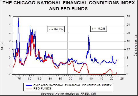
Although there are several financial conditions indexes, we prefer the one generated by the Chicago Federal Reserve Bank. This index has 105 variables, including various interest rate spreads, volatility measures, and the levels of several indexes and interest rates. The index is updated weekly. A rising index suggests increased financial stress (deteriorating financial conditions). From 1973, when the index began, to mid-1998, there was a tight correlation between the level of fed funds and financial conditions. For the most part, policymakers could use financial conditions as a “force multiplier” to enhance policy. When the policy rate rose, financial conditions worsened in lockstep. When the policy eased, they rapidly relaxed.
But, after mid-1998, the two data series became almost uncorrelated. What happened? A couple of factors likely affected this relationship. The first was the passage of the Gramm-Leach-Bliley Act, which eliminated the difference between commercial and investment banking. This bill changed the financial system, leading to more financial activities occurring outside the traditional banking system. In other words, the non-bank banking system was fostered by this bill. Why is that important? To illustrate, instead of borrowing from a bank, firms could issue debt or do collateralized borrowing in a much less regulated environment. Raising the policy rate didn’t necessarily lead to reduced borrowing because the financial markets have more ways to provide liquidity due to the changes in regulation.
The second factor was greater transparency in monetary policy. Even in the late 1980s, the FOMC acted in secret. “Fed watchers” tried to divine if a policy change had occurred by monitoring money supply data or bank reserve changes. But by the mid-1990s, the FOMC started announcing when the policy rate changed, and over the years, it has been increasingly transparent about its policy expectations. In general, society tends to treat transparency as a good unto itself. But by making its policy direction clear, markets could adjust and thus had little to fear from “surprises.” In the non-bank banking system, participants could use derivatives to insulate their positions from policy changes, rendering them less effective.
So, due to changes in the financial markets and increased openness, the FOMC has lost its ability to use financial conditions as an effective policy tool. For example, on the above chart, the FOMC steadily lifted rates from 2004 to 2006. During this time, financial conditions didn’t move. Then, in 2007-08, when financial conditions deteriorated rapidly, aggressive rate cuts had little ability to improve them. It took years of “zero-rate policy” and rounds of Quantitative Easing (QE) to finally improve financial conditions to a level in line with the pre-Great Financial Crisis period.
Recent history shows that when financial conditions weaken, it takes aggressive and swift action by the FOMC to reduce it. In March 2020, financial conditions deteriorated rather quickly, and not only did the FOMC cut rates rapidly, but it implemented a broad intervention into the financial markets to support their function. In addition, the balance sheet was expanded at a pace not seen outside of wartime. Clearly, the pandemic was part of the policy response, but widening credit spreads and other signs of financial stress were also part of the Fed’s actions.
Although the call for purposely undermining financial conditions is understandable, the above chart shows it could trigger unforeseen outcomes. We are no longer in a world where financial conditions deteriorate in lockstep with changes to the policy rate. Instead, over the past 24 years, these conditions have shown a tendency to ignore policy tightening, only to deteriorate rapidly with little warning. A modest weakening of financial conditions might be welcome, increasing the potency of tighter policy. However, a sudden spike, as seen in 2008 and 2020, could be destabilizing, forcing the FOMC to rapidly reverse its current policy path. Sadly, such events are almost impossible to predict in advance, although we can say that they seem to occur after tightening cycles.
It is possible that 2008 and 2020 may reflect the immaturity of the non-bank financial system, and markets may have evolved to a point where such market events have become less likely. The backstops offered by the Fed during March 2020 might serve as a blueprint for containing financial crises. Therefore, allowing financial conditions to deteriorate is less risky. However, it appears to us the burden of proof lies with proving that tightening won’t “break something.” And so, we remain vigilant, watching for funding issues that could trigger a run on liquidity and force the FOMC to ease.