by Asset Allocation Committee

There are three factors that tend to cause recessions—inventory misadjustments, policy errors and geopolitical events.  The first in the series has become less of a factor over time.  Inventory management has improved dramatically since the end of WWII, and excess inventory leading to falling output has become less of an issue.  Therefore, we tend to focus on the latter two factors.  Since fiscal policy changes tend to occur more slowly, monetary policy is where we spend most of our efforts.  With regard to geopolitical events, we write a weekly report on that issue.

Monetary policy is facing a serious signaling problem.   One of the signals we use for monetary policy is the implied LIBOR rate from the two-year deferred Eurodollar futures.  That rate is an indication of what the financial markets are thinking.  As we will show below, it has generally been a good indicator for when policy tightening should stop.  The implied LIBOR rate has declined significantly.

Since peaking at 3.30% last October, the rate has declined to 1.90%, a drop of 140 bps.

The lower lines show the implied LIBOR rate with the fed funds target.  Note that the FOMC has tended to stop raising rates when the spread inverts.  During the Greenspan years, easing tended to follow shortly after inversion.  The Bernanke Fed did stop raising rates after inversion but didn’t ease, which may have contributed to the severity of the 2007-09 recession.

To compare how the financial market signs compare to economic signals, we have overlaid the fed funds target/deferred LIBOR rate with two of the Mankiw Rule variations, one using core CPI and the unemployment rate and the other using core CPI and the employment/population ratio.  The Mankiw Rule is a simplified version of the Taylor Rule, which estimates the fed funds rate based upon core inflation and GDP relative to potential GDP.  Because potential GDP isn’t directly observable, Mankiw’s original research replaced GDP with the unemployment rate.  We have created our own variations as well (not shown).

The lower lines on the chart show the implied LIBOR rate, with the fed funds target and the two aforementioned estimated Mankiw Rule rates.  Aside from the Mankiw Rule variation using the unemployment rate, all other variations are suggesting the Fed should be cutting rates.  However, in each of the prior inversion events (shown by the vertical lines on the above chart), the estimates for the fed funds target from the Mankiw Rule variations were below the target rates.

This has been a consistent issue during this expansion; essentially, it has been difficult to determine the degree of slack in the economy.  Fortunately for policymakers, this problem of estimating slack has not been a serious issue until recently.  Given the current divergence in signals, the most likely outcome is for the FOMC to maintain a steady posture.  The lack of a clear signal between the financial markets and the interest rate markets increases the odds of a policy mistake.  Although the FOMC’s official stance is neutral, we suspect the next move will be to lower the policy rate.

View the PDF

by Asset Allocation Committee

How important have mergers, buybacks, etc. been to equity market performance?  Several analysts have attempted to answer this question by focusing on buybacks alone.  However, there is a more straightforward method of looking at this question and including all the factors that affect the number of shares available—the index divisor.

This chart shows the divisor for the S&P 500.

The divisor adjusts the S&P for membership changes (either by mergers or index adjustment), new share issuance or repurchases, or special stock-related transactions.  So, it isn’t a pure look at buybacks but isolating buybacks alone may overstate the impact of the activity if new shares are being issued or it may ignore the impact of membership adjustments.  In general, a rising divisor tends to depress the index and vice versa.  In the most recent data, the divisor peaked in Q3 2011; the decline in the divisor is partly due to buybacks, but merger activity has affected it as well.

To calculate the impact of the divisor, we would use the following formula:

Divisor * S&P Index = S&P Market Capitalization

Rearranging terms leads to this formula:

S&P Index = S&P Market Capitalization/Divisor

And so, if we take the market capitalization and hold the divisor fixed at this peak in Q3 2011, we can estimate what the S&P 500 would have been without the decline in the divisor.

At the end of Q1, the S&P 500 was at 2824.44; if the divisor had held at its previous peak, it would have been 2593.63, or 8.2% lower.

The more important question is if or when the trend in the divisor might reverse.  In general, history suggests that elevated equity market values tend to trigger equity issuance.  However, that has not been the case since 2000.

This chart shows the divisor and the S&P 500 Index since 1964.  From that year to Q1 2000, the two series were positively correlated at the 69.5% level.  However, since then, the correlation between the two series has not only flipped to inverse but strengthened.  During this century, for the most part, the equity markets appear less critical to raising capital.  Overall, we expect the divisor to continue to decline as firms continue to shrink the number of shares available; if we are correct, the equity markets have a modest tailwind going forward.

View the PDF

by Asset Allocation Committee

Foreign exchange economics has become something of a backwater in economic theory.  There are four predominant valuation methodologies; if one were any good, the others wouldn’t exist!  The four are purchasing power parity, real equilibrium theory, interest rate differentials and productivity equalization (unit labor cost equalization).   The general idea is that under flexible exchange rates, currency values adjust to eliminate differences between nations.  The oldest of the four is purchasing power parity, which assumes exchange rates move to equalize prices across nations.  Real equilibrium theory suggests the exchange rate adjusts to equalize real current account differences.  Interest rate differentials suggest the exchange rate adjusts to equalize interest rates, and productivity equalization normalizes unit labor costs (labor costs adjusted for productivity) across nations.

In practice, the macro data used to calculate fair value for exchange rate models is usually not granular enough to capture differences between nations.  For example, with purchasing power parity, all goods and services in an inflation index are not tradeable and so these non-traded products cannot be adjusted via exchange rates.  And so, all the models tend to be useful only at extremes.  In other words, wide deviations from calculated fair value can offer useful signals, but, like all valuation models in finance, they are not helpful for timing.[1]  At the same time, long-term investors can find value in such models in that they do signal when a relationship is cheap or rich.  This is helpful but only if (a) the investor is truly patient, and (b) something significant hasn’t changed.

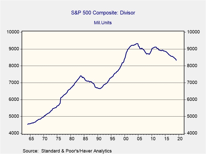
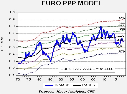
Our favorite model is purchasing power parity because long-term inflation histories are usually easy to access and, theoretically, inflation is a very important variable.  As we have been noting for some time, the dollar is expensive based on these models.  For example:

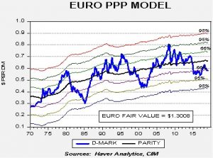
This is a parity model for the EUR, using German inflation against U.S. inflation.  The fair value exchange rate is $1.3008 compared to the current rate of $1.1200.  This deviation from fair value, which in historical ranges is where reversals usually occur, has led to the belief that, at some point, the dollar will weaken.  The model also suggests that once a reversal occurs it is common that the exchange relationship will overshoot.  Thus, a turn in the exchange rate is an important event; in markets, for U.S. investors, foreign stocks and commodities are two areas where one can historically find outperformance.

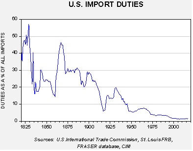
But, the Trump administration has moved to the use of tariffs to combat persistent trade deficits.  The use of tariffs had fallen out of favor, in part because the U.S. fostered open trade, and because tariffs tend to be less effective under flexible exchange rates.  Why?  Because the nation targeted by tariffs can simply allow its currency to weaken, offsetting the price effect of the tariff.  For example, if China is a target for tariffs, the expected response would be CNY depreciation.

This chart shows how tariffs have become less of a factor.

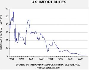
As the chart shows, after the 1920s, the U.S. has steadily abandoned tariffs…until now.

If the administration continues down this path of using tariffs on a widespread basis, our position on future dollar weakness has to be reconsidered.   Although the tariff policy may not last once Trump leaves office, one cannot necessarily assume that to be the case.  Of course, the U.S. could act against depreciation too, but that might prove difficult to stop.

At some point, we expect the administration (or some future administration) to realize that tariffs are a poor tool for reducing the trade deficit.  Currency weakness is more effective but the most effective method is capital controls.  The reason the U.S. runs persistent trade deficits is because the dollar is the reserve currency.  If the U.S. denied access to the U.S. capital markets, then foreigners would have less reason to engage in policies to promote exports.  Would there be collateral damage from such policies?  Yes, but we may be approaching a point where Americans are willing to accept those side effects in order to reduce inequality and lift domestic wages.

View the PDF

[1] Or, said another way, “markets can stay stupid longer than you can stay solvent.”

by Asset Allocation Committee

While the financial industry is rife with performance comparisons to selected benchmarks, the most important investing goal for the majority of clients is a return above inflation that avoids catastrophic losses.  Although beating the S&P 500 is a nice goal, solely focusing on that outcome may lead an investor to accept more risk than appropriate.  This is an age-old issue where one confuses ends with means.  Benchmarking is a means to an end.  A benchmark gives investors some insight into how their investments are doing but should never be considered an end in itself.  Sadly, measurement of performance seems to have eclipsed, and even replaced, the principal goals for clients.  In other words, the benchmark has become the goal.

A good example of the problem with benchmarking is found in academia.  Students have been told that the “4.0” is the clear marker of academic success.  Now, getting all “As” is a good thing.  But, anyone who has been to college knows that the GPA can be gamed.  Students can fill their electives with easy courses.  They can select the easiest professors in their major’s hardest courses.  And, they can cheat.  Or, perhaps equally as perverse, they can “know it for the test.”  In other words, they can memorize the necessary information but fail to really understand it.  Resolving this issue is part of hiring new graduates.  There are ways to ferret out who knows their stuff and who gamed.  Checking transcripts is a good way to look for clues—what were the electives and how did the candidate do in the hard classes?  Another is to ask questions about the most basic components of a discipline but in a way that is rarely presented in class.  An example for economists is, “Assume all drug users are addicts; what is the best way to reduce illicit drug consumption?”[1]  However, how many positions are filled by candidates who are screened by GPA?  In other words, how many good candidates never get an interview because their GPA fell below 3.5 because they took more challenging course work?

Let’s suppose that instead of attempting to help clients accumulate wealth within their acceptable risk tolerance, the goal was to outperform the S&P 500 Index and the criteria was what outperformed the index over the past seven calendar years.  Out of the 34,468 U.S. dollar-based indices in Morningstar’s database, the sole index that met this criteria was the S&P HealthCare Equipment Select Industry Index.  Naturally, exposure exclusively to this single index would be a poor investment strategy for the vast majority of clients, as it would expose them to very specific risks, yet it underscores the notion that simply striving to outperform the return of a particular index is fraught with the potential risk of a permanent impairment of capital.

Another problem that arises in making relative performance the principal objective is the potential for miscreants to juggle benchmarks in order to appear successful.  As an example, the table below illustrates the divergence that is associated with popular small cap growth benchmarks.  While all four of the benchmarks in the table are from highly reputable providers with well-documented methodologies for the U.S. small cap growth stocks included in their indices, the variance among these four in any given year can be profound.  Note that even with indices from the same vendor the differences can be significant as evidenced by the MSCI U.S. Small Cap Growth Index varying from the MSCI U.S.A. Small Growth by 244 basis points in 2018.

A further complication that may be encountered is the utilization of benchmarks that incorporate significant complexity in the myriad sub-asset classes that roll up to major asset classes.  The resulting information will be a hash of statistics that are of little use to either investors or advisor supervision.

These potential pitfalls do not obviate the necessity of monitoring and evaluating relative performance as part of proper due diligence.  The evaluation of a manager’s portfolio or asset allocation strategy against an appropriate benchmark is an essential tool for validation of an investment thesis, which can lead to the achievement of the client’s goals.  However, this can be taken to extremes.  Our industry’s all-consuming fascination with performance measurement has the potential to cause actions that are perpendicular to the goal of inflation-adjusted wealth creation, such as performance chasing.

What, then, is the correct approach to ensure a manager is properly positioned in a client’s portfolio or an asset allocation strategy is appropriate to help attain the client’s goal?  The most straightforward means is to evaluate a manager or asset allocation strategy against a benchmark that is objective, possesses a sound methodology, recognizable, germane to the asset class represented and free of unnecessary complexity.  For this last facet, the notion of Occam’s razor applies.  This approach will naturally yield significant tracking error; however, tracking error should not only be expected, but embraced, for an active manager.  While on a quarter-to-quarter basis investors may observe divergent returns relative to the benchmark, during discrete, representative periods and especially through a full market cycle, an uncomplicated and recognizable benchmark will represent a solid barometer against which to measure the risk-adjusted return of a manager or investment strategy.  This will serve to evaluate whether the manager or strategy is contributing to the overarching client goal.  But, ultimately, the key point to remember is that a benchmark is a means to an end, not an end in itself.

View the PDF

[1] If all users are addicts, then the demand curve is highly inelastic.  Reducing supply merely drives up the price, but reducing demand (drug rehab, substitution) could reduce demand and have the biggest effect on reducing consumption.