Asset Allocation Weekly (June 23, 2017)

by Asset Allocation Committee

The FOMC did raise rates at the June meeting, which was fully expected.  The dots chart suggested that we would see one more hike this year and three next year.  In addition, the central bank gave some indication of how it would shrink its balance sheet.  Although the statement didn’t signal when the reduction would begin, Chair Yellen indicated in the press conference that it would begin before year’s end and seemed to hint it may start much sooner than the market expects.

In this report, we want to examine two concerns we have about the path of policy tightening.  The first concern is the level of the policy rate.  To measure the impact of the policy rate, we use the Mankiw Rule.  The Mankiw Rule models attempt to determine the neutral rate for fed funds, which is a rate that is neither accommodative nor stimulative.  Mankiw’s model is a variation of the Taylor Rule.  The latter measures the neutral rate using core CPI and the difference between GDP and potential GDP, which is an estimate of slack in the economy.  Potential GDP cannot be directly observed, only estimated.  To overcome this problem with potential GDP, Mankiw used the unemployment rate as a proxy for economic slack.  We have created four versions of the rule, one that follows the original construction by using the unemployment rate as a measure of slack, a second that uses the employment/population ratio, a third using involuntary part-time workers as a percentage of the total labor force and a fourth using yearly wage growth for non-supervisory workers.

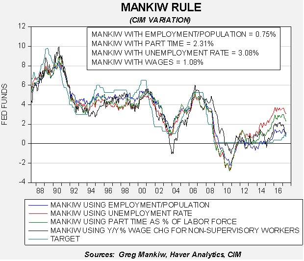
Using the unemployment rate, the neutral rate is estimated at 3.08%.  Using the employment/population ratio, the neutral rate is 0.75%.  Using involuntary part-time employment, the neutral rate is 2.31%.  Using wage growth for non-supervisory workers, the neutral rate is 1.08%.

The labor data has been mixed during this recovery.  The unemployment rate has fallen sharply, but other measures, most notably the employment/population ratio, have fallen much more slowly.

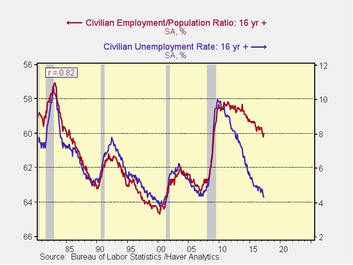
If the relationship between the unemployment rate and the employment/population ratio that existed from 1980 through 2010 had remained the same, the current unemployment rate would be closer to 7.5%.  Using the above Mankiw Rule with a 7.5% unemployment rate and the current core inflation rate would generate a neutral policy rate of -0.61%!  In other words, not only would the FOMC not be tightening, but cutting the balance sheet wouldn’t be considered either.

The conventional wisdom is that the employment/population ratio is being affected by retirements and thus the labor market slack isn’t as great as that indicator would suggest.  However, we note that wage growth is much more consistent with the employment/population ratio than the unemployment rate.  Thus, there is a legitimate worry that the Fed may overtighten and put the economy at risk.  Currently, the financial markets only expect one more tightening over the next two years; if the dots plot is the path of policy, the odds of a recession will rise.

If the employment/population ratio is the accurate measure of slack, we are already 37 bps above neutral.  Policy would be tight at 100 bps.  Thus, we are two to three hikes from putting the economy at risk.  Of course, the ratio could improve or inflation could rise, but without those events occurring, the risk to the economy from tighter monetary policy is rising.

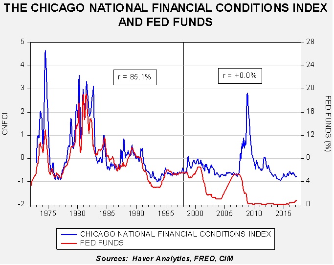
The second concern is the balance sheet.  The actual effect of QE on the economy is difficult to determine.  We tend to think that the most likely impact was that the balance sheet expansion confirmed that the Fed was determined to execute an easy policy even with the policy rate at zero.  The level of the balance sheet appears to have had a strong effect on investor sentiment.

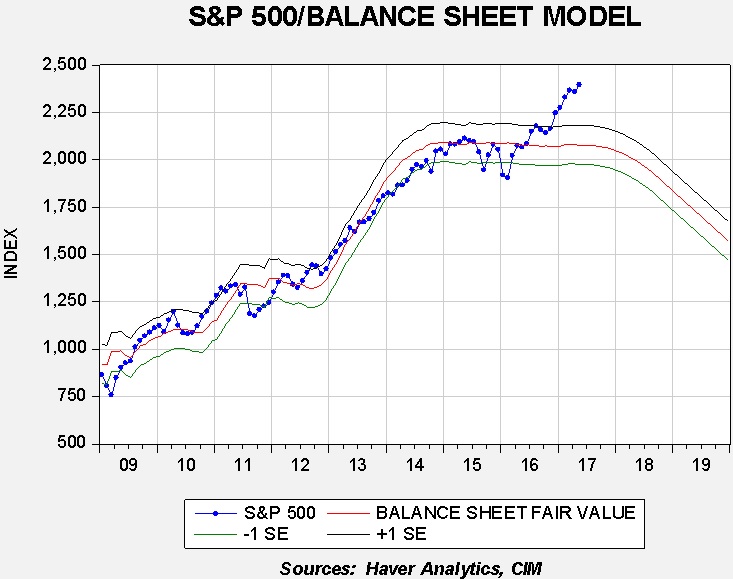
This chart forecasts the S&P 500 by using the size of the balance sheet.  From 2009 into late last year, this equity index closely followed the balance sheet.  After the election, equities shifted focus toward expectations of tax reform and fiscal expansion.

We have extended the forecast generated from the balance sheet using the FOMC’s stated plan for reducing the balance sheet and assuming the reduction begins in September.  The Fed intends to start slowly, only $10 bn per month, reaching $50 bn after a year.  It is obvious that the balance sheet could become a headwind by 2018.  This above chart isn’t our forecast for equities but it does suggest that the combination of rate hikes and balance sheet reductions is signaling that monetary policy will tend to become a headwind for equities.  If the Trump administration fails to move forward with tax reform or infrastructure spending, equity markets will be vulnerable to a correction.

View the PDF

Weekly Geopolitical Report – The Second Korean War: Part I (June 19, 2017)

by Bill O’Grady

Tensions with North Korea have been escalating in recent months.  The regime has tested numerous missiles and claims to be capable of building nuclear warheads, which, combined with an intercontinental ballistic missile (ICBM), would make the Hermit Kingdom a direct threat to the U.S.  Such a situation is intolerable to the U.S., and thus there is rising concern about an American military response.

In Part I of this report, we will recap the Korean War, focusing on the lessons learned by all sides of the conflict.  We will discuss North Korea’s political development through the postwar period and the fall of communism.  This examination will frame North Korea’s geopolitical situation.  The next step will be to analyze U.S. policy with North Korea and why these policies have failed to change the regime’s behavior.

In Part II, we will use this backdrop to discuss what a war on the peninsula would look like, including the military goals of the U.S. and North Korea.  This analysis will include the military assets that are in place and the signals being sent by the U.S. that military action is under consideration.  War isn’t the only outcome; stronger sanctions and a blockade are possible, and the chances of success and likelihood of implementation will be considered.  As always, we will conclude with market ramifications.

View the full report

Asset Allocation Weekly (June 16, 2017)

by Asset Allocation Committee

Last week, the Federal Reserve published its Financial Accounts of the United States report, more commonly called the “Flow of Funds” data.  The report offers a plethora of insights into the economy.  This week we want to examine the household debt situation.

In Q1, household debt reached $15.1 trillion, up 3.4% from the previous year.

Although the growth in liabilities is positive for consumption, note that the current growth rate is well below the 9.8% average from 1946 through 2006.  As we will show below, deleveraging continues but the pace has slowed dramatically.  Still, part of the reason for sluggish growth is that households are simply not borrowing as quickly as what we have seen in the postwar period.

As noted, deleveraging has continued but the pace has slowed to a crawl.

Household debt (non-profit debt is not meaningful) is down to 78.2% of GDP after peaking at 97.7%.  It is virtually impossible to determine the “correct” or sustainable level of debt, but a solid case can be made that any reading above 60% is probably not manageable over the long run.  Of course, there are three ways this ratio can decline, falling levels of debt, rising real GDP relative to debt or rising inflation relative to debt.  The lack of inflation has probably prevented an even larger drop in this ratio.

Low interest rates have reduced the servicing costs.

This chart shows household debt service costs as a percentage of after-tax income.  Debt service costs rose steadily from 1993 into 2007.  The combination of falling interest rates and the level of debt has led to a sharp drop in debt service costs.  At these levels of debt service, one would expect that households would be encouraged to expand their debt levels.  However, the “hangover” from the debt crisis has not yet diminished.

As long as households are reluctant to borrow, economic growth will remain slow and inflation low.  This combination should lead to moderate policy tightening from the FOMC and an extended business cycle.  If borrowing were to increase, these conditions might change but, for the foreseeable future, we expect borrowing to remain sluggish and economic growth to remain weak as well.

View the PDF

Weekly Geopolitical Report – South Korea’s Too Big to Fail (June 12, 2017)

by Thomas K. Wash

On March 10, Park Geun-hye was removed from her position as president of South Korea. Her ouster came on the heels of a scandal involving her close confidant who is accused of seeking bribes from chaebols, a group of family-owned multinational conglomerates that dominate the South Korean economy, to curry favor with the Park administration. Prior to the scandal, Park’s political party, Liberty Korea, had been accused of prioritizing the interests of the chaebols over the interests of the Korean people.

This controversy has paved the way for populist candidate Moon Jae-in, from the Democratic Party of Korea, to rise to the presidency. It is assumed that he will look to loosen government ties with chaebols. Recently, chaebols have come under scrutiny as many people feel that their overall size and dominance have constrained the economy. Currently, South Korea suffers from high youth unemployment, rising household debt and rising income inequality. Moon Jae-in has vowed to tackle each of these problems in addition to chaebol reform. This task may prove to be difficult as the chaebols have accumulated a lot of political clout over the years, thus he may find it difficult to pass serious reforms through parliament.

In this report, we offer a brief history on the origins of chaebols and their influence in lifting the country out of poverty. From there, we will focus on the role the Asian Financial Crisis played in changing public attitude toward chaebols and examine possible chaebol reforms. Finally, we will conclude with market ramifications.

View the full report

Asset Allocation Weekly (June 9, 2017)

by Asset Allocation Committee

We have been monitoring the S&P 500 performance relative to new GOP administrations.  Based on the historical pattern, the market has reached the average peak level a few weeks early.

This chart shows the performance of the S&P 500 on a weekly close basis, indexed to the first Friday of the first trading week in the year of the election.  We have averaged the first four years of a new GOP president.  So far, this cycle’s equity market has generally, though not perfectly, followed the average.  Based on that pattern, the current level of the market is around the usual peak.  Clearly, this election cycle could be different, but the average does suggest we could be poised for a period of weakness.

So, what might cause a pullback?  Here are a few candidates:

A debt ceiling crisis: The Treasury indicates that the government may begin to shut down as early as August if the debt ceiling isn’t lifted.  With the GOP controlling Congress and the White House, raising the debt limit should be perfunctory.  However, there are rumblings that the Freedom Caucus will demand spending cuts to agree to any debt limit increases.  The Democrats, after watching President Obama deal with two government shutdowns and the sequester over the debt limit, are in no mood to work with the administration and may force the congressional leadership to deal with the Freedom Caucus.  If another debt limit crisis triggers a new government shutdown and raises fears of a potential downgrade of Treasury debt, a pullback in equities would likely result.

Winds of war on the Korean Peninsula: The U.S. will have three carrier groups in the East China Sea in the coming weeks.  Although we doubt the Trump administration wants a war with North Korea, the U.S. is putting enough assets in the region to go to war if it so decides.  A full-scale attack on North Korea would be a bloody affair; the Hermit Kingdom has been preparing for such an attack for years and even if its nuclear program isn’t ready to deliver a weapon, its conventional forces will wreak havoc on the South.  Even a hint of a conflict will likely prompt a pullback in risk assets.

Monetary policy worries: The FOMC appears driven to raise the fed funds target rate.  As we have noted before, there is a good deal of uncertainty surrounding the degree of slack that remains in the economy.  The FOMC appears to be leaning toward the notion that the economy is getting close to capacity and further declines in unemployment will surely lead to inflation rising over target.  Although financial markets didn’t react well to the rate hike in December 2015, the subsequent increases have occurred without incident.  Telegraphing the increases has reduced the risk to rate hikes but the odds of overtightening will increase if the Federal Reserve has miscalculated the level of slack in the economy.  This potential concern, coupled with plans to begin reducing the size of the balance sheet later this year, could begin to undermine market sentiment.

We want to note that the average decline shown on the above graph is not a numerical forecast; we tend to view the direction as a more important indicator than level.  It suggests that a period of equity market weakness is a growing possibility later this summer.  What we don’t see, at least so far, is evidence of anything more than a pullback.  Recessions tend to be the primary factors that lead to bear markets.  The economy is doing just fine; the yield curve hasn’t inverted, the ISM manufacturing index is comfortably above 50 and there hasn’t been any evidence in the labor markets to suggest a drop in economic growth.  Thus, we may see a weak summer for stocks but nothing that would lead us to take a defensive position in the equity markets.  Instead, a pullback will likely create an opportunity for investors.

View the PDF

Weekly Geopolitical Report – Are the Germans Bad? (June 5, 2017)

by Bill O’Grady

At the NATO meetings late last month, the German media reported that President Trump had called the Germans “bad” for running trade surpluses with the U.S.  The president threatened trade restrictions, focusing on German automobiles.  Needless to say, this comment caused a minor international incident.

Although such incidents come and go, it did generate a more serious question…are German policies causing problems for the world?  In this report, we will review the saving identity we introduced in last month’s series on trade and discuss how Germany has built a policy designed to create saving.  We will move the discussion to the Eurozone and show the impact that German policy has had on the single currency.  From there, we will try to address the question posed in the title of this report.  We will conclude, as always, with market ramifications.

The Saving Identity
In the month of May, we published a four-part report on trade that is now combined into a single report.[1]  In that report, we introduced the saving identity.

(M – X) = (I – S) + (G – Tx)[2]

The saving identity states that private sector domestic saving (I – S) plus public sector saving (G – Tx) is equal to foreign saving.  If a country is running a positive domestic savings balance, either by investing less than it saves or by running a fiscal surplus, it will run a trade surplus (X>M).  In public discussion, trade appears to be all about jobs, relative prices, trade barriers, etc.  However, regardless of how nations interfere with trade, the saving identity will always be true.  As we noted in the aforementioned report, tariffs, exchange rate manipulation and administration barriers will, in the final analysis, be explained through the saving identity.

In the process of economic development, nations must build productive capacity through investment.  Both public and private investment are necessary for success.  Public investment in infrastructure, roads, bridges, canals, etc., are critical to supporting private investment.  In capitalist societies, a legal framework to adjudicate contract disputes and support the enforcement of agreements is also necessary and mostly provided by the public sector.  Private investment usually occurs along with public investment.  But, all investment requires funding, which comes from saving.  That saving can come from both domestic and foreign sources.

View the full report

___________________________________

[1] See WGR, Reflections on Trade (full), May 2017.

[2] Imports (M), exports (X), investment (I), saving (S), government consumption (G) and taxes (Tx).

Asset Allocation Weekly (June 2, 2017)

by Asset Allocation Committee

In the last FOMC minutes, policymakers signaled another hike at the upcoming June 14th meeting.  We continue to closely monitor financial conditions but, so far, financial markets are rather sanguine about the impact of policy tightening.

The blue line on the chart shows the Chicago FRB Financial Conditions Index, which measures the level of stress in the financial system.  It is constructed of 105 variables, including the level of interest rates, credit spreads, equity and debt market volatility, delinquencies, borrower and lender surveys, debt and equity issuance, debt levels, equity levels and various commodity prices (including gold).  A rising line indicates increasing financial stress.  The red line is the effective fed funds rate.  Until 1998, the two series were positively and closely correlated.  When the Fed raised rates, financial stress rose; when the Fed lowered rates, stress declined.

We believe there are two factors that changed this relationship.  The first is policy transparency.  Starting in the late 1980s, the Fed became increasingly transparent.  For example, before 1988, the FOMC would meet but issue no statement about what it had decided to do.  Investors and the financial system had to guess whether policy had been changed.  Starting in 1988, the central bank began publishing its target rate.  In the 1990s, it began issuing a statement when rates changed.  Eventually, a statement followed all meetings.  As the FOMC has become more transparent, the correlation between stress and the level of fed funds has changed.  Essentially, the markets now know with a high degree of certainty when rate changes are likely.  This is especially true of tightening.  The FOMC appears to avoid making rate hikes that surprise the market.

The second factor is financial system stability.  From the Great Depression into the 1980s, policymakers put a high premium on system stability at the expense of efficiency.  Bank failures were rare and there were a large number of rather small institutions.  In addition, commercial banks were separated from investment banks.  The drive to improve efficiency led to consolidation among commercial banks and a breakdown of the barriers between commercial and investment banks.  Although this made the system more efficient, it also undermined stability.  Thus, when raising rates, the Fed must pay close attention to system stability to prevent crises, which has tended to lead to gradual and measured policies; this behavior maintains stability…until it doesn’t!

Essentially, policymakers and investors face the Minsky Paradox; the more stable markets become the more risks investors take, leading to conditions that cannot be sustained.  Unfortunately, it’s hard to know in advance when rate hikes become problematic.  It is likely that as rates rise, factors that may have been manageable at lower rates become dangerous at higher rates.  Those conditions can change faster than policymakers can likely react.  For now, there isn’t much evidence of trouble but the fact that policy is tightening raises the likelihood, however small, that problems could develop.

View the PDF

Asset Allocation Weekly (May 26, 2017)

by Asset Allocation Committee

The dollar is in its third major bull market since currencies began floating in 1971.

This chart shows the JPM dollar index which adjusts for relative inflation and trade.  The previous two bull markets exhibited greater strength than the current one.  Because of the dollar’s reserve currency role, there will always be an underlying demand for dollars for foreign reserve purposes.  Thus, U.S. policymakers can run fiscal deficits and tax policies that penalize saving (for example, we tax income instead of consumption) and not suffer from foreign exchange crises.  At the same time, dollar strength can act as a drag on the economy; it tends to make imports more attractive and can undermine the competitiveness of domestic firms.

The previous two dollar rallies were tied to specific fundamental factors.  The 1978-85 bull market was mostly attributable to the Volcker Federal Reserve.  Paul Volcker instituted monetary policy based on money supply growth instead of interest rate targets.  This allowed interest rates to rise to extraordinary levels (fed funds peaked at 19.1% in June 1981) and made the dollar very attractive.  The 1995-2002 bull market was mostly caused by productivity gains, although fiscal surpluses likely contributed as well.  Technology investment began to boost the economy in the latter half of the 1990s and made the U.S. an attractive investment venue.  The surplus reduced available Treasuries and made it difficult to build reserves without bidding the dollar higher.  The current bull market is similar to the Volcker bull market in that it appears to be mostly due to monetary policy.  The Federal Reserve began to reverse its unconventional monetary policy measures before the other major G-7 economies, boosting the greenback.

Valuing currencies is difficult as it is generally true that the currency markets focus on different factors over time.  There are periods when relative inflation is dominant.  During other periods, the external accounts drive the exchange rates, while other times interest rate differentials are key.  The valuation model with the longest history is purchasing power parity, which is based on relative inflation rates.  The thesis is that the exchange rate should act to balance prices between nations and so a country with higher inflation relative to another should have a weaker exchange rate to unify prices across countries.  In practice, we find that not all goods are tradeable, inflation indices are not the same across countries and relative pricing parity models don’t account for capital flows.  Although parity models often deviate from fair value, they can be useful when parity reaches an extreme.

This chart shows the German/U.S. parity model, which uses CPI from Germany and the U.S. to establish parity.  Currently, the exchange rate is nearly two standard errors below parity, meaning the D-mark (or the euro) is undervalued relative to the dollar.  As the chart shows, the exchange rate rarely stays around purchasing power parity.  However, when it reaches the two-standard error level in either direction, it usually means the exchange rate will eventually reverse.  It isn’t uncommon for the exchange rate to remain over or undervalued for a long period of time.  However, we eventually do see a reversal from extreme levels.  Usually, there is a catalyst that brings an adjustment to valuation.  In 1985, it was the Plaza Accord which was specifically designed to weaken the dollar.  The end of the second bull market was likely due to the end of the tech bubble in equities and the Bush tax cuts, which reduced the fiscal surplus.

It appears we are seeing two catalysts that may be signaling the end of this dollar bull market.

The reversal of monetary policy: The dollar initially rallied on the divergence of monetary policy.  The Federal Reserve was ending QE and beginning to raise rates, while the Bank of Japan (BOJ) was expanding QE and the European Central Bank (ECB) was implementing QE and experimenting with negative interest rates.  This kicked off the current dollar bull market that began in mid-2014.  Although the FOMC is planning to raise rates further that action has been well telegraphed.  At the same time, it appears the ECB is poised to raise rates and end its QE program.  And, European economic growth has been strengthening, which will likely accelerate policy tightening.  Even the BOJ is considering easing some of its support.  Given the degree of dollar overvaluation, foreign policy tightening will likely weaken the dollar in the coming months.

Political turmoil is favoring foreign currencies: There is no lack of political turmoil in the developed countries.  We have had two major elections in Europe thus far, with upcoming German elections in the fall and Italian elections expected in February.  Brexit continues to roil Europe.  Tensions are rising in the Far East as North Korea continues to test missiles and threaten its neighbors.  When President Trump won the election in November, the dollar rose on expectations of trade restrictions, tax reform that would support repatriation and infrastructure spending which would boost growth.  As the Trump administration has gotten sidetracked on other issues, these expectations have dwindled.  Even though political risk remains high throughout the developed markets, the high dollar valuation and disappointment surrounding the president’s policies appear to be undermining the dollar.

If the dollar’s bull market is coming to a close, what can we expect?  First, it gives a tailwind to foreign investment.  Emerging markets, which have been strong this year, would likely receive further support if the dollar begins to weaken.  Second, commodities would benefit.  For example, our oil inventory/EUR model for oil prices indicates that a €1.30 would generate a fair value for oil near $78 per barrel, even with the current elevated level of inventories.  Gold prices are traditionally supported by dollar weakness as well.  The asset allocation committee will be weighing the likelihood of dollar weakness and take appropriate measures in the coming months.

View the PDF

Weekly Geopolitical Report – Reflections on Trade: Part IV (May 22, 2017)

by Bill O’Grady

(Due to the Memorial Day holiday, our next report will be published on June 5.)

This is the final report of our four-part series on trade.  This week, our discussion on trade continues with a look at the relationship between trade, employment and inflation.  We will also conclude the series with market ramifications.

What are the tradeoffs of trade?
Trade is part of a broader societal tradeoff between equality and efficiency.[1]  To function, societies need some degree of both.  Nations with a high level of inequality tend to become politically unstable.  At the same time, perfect equality tends to stifle initiative and prevent the building of productive capacity.  Efficiency helps an economy provide goods and services at reasonable costs.  Complete inefficiency makes everyone poor.

Okun’s insight is that societies balance equality and efficiency to maintain order.  What we observe in history is that there doesn’t appear to be a balance point; in other words, this isn’t an optimization problem.  Instead, we see broad periods of oscillation where one goal or the other is waxing or waning.

View the full report

___________________________________

[1] Okun, A. (1972). Equality and Efficiency: The Big Tradeoff. Washington, D.C.: Brookings Institute.