The business cycle has a major impact on financial markets; recessions usually accompany bear markets in equities. We have created this report to keep our readers apprised of the potential for recession, which we plan to update on a monthly basis. Although it isn’t the final word on our views about recession, it is part of our process in signaling the potential for a downturn.
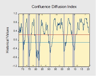
In March, the diffusion index nearly fell into recession territory. The weakness in the report was primarily due to the coronavirus pandemic, turmoil in the financial markets and the Saudi-Russia oil dispute. Last month, confirmed cases of COVID-19 in the U.S. rose from 74 at the start of the month and grew to over 180,000. Meanwhile, the oil price war between Saudi Arabia and Russia led oil prices to fall to a near-20-year low. As a result, equities dropped and Treasuries rallied. The interest rate on the 10-year T-note fell below 1.0% for the first time ever. Additionally, the manufacturing sector showed mixed signals as a slowdown in delivery times reflected positively in the report despite a drop in new durable goods orders. The employment numbers were abysmal and will likely be worse in next month’s report. In this report, six out of the 11 indicators were in recession territory. The reading for March fell to +0.333 from +0.57, a hair above the recession signal of +0.250.
The chart above shows the Confluence Diffusion Index. It uses a three-month moving average of 11 leading indicators to track the state of the business cycle. The red line signals when the business cycle is headed toward a contraction, while the blue line signals when the business cycle is headed toward a recovery. On average, the diffusion index is currently providing about six months of lead time for a contraction and five months of lead time for a recovery. Continue reading for a more in-depth understanding of how the indicators are performing and refer to our Glossary of Charts at the back of this report for a description of each chart and what it measures. A chart title listed in red indicates that indicator is signaling recession.
by Bill O’Grady, Thomas Wash, and Patrick Fearon-Hernandez, CFA
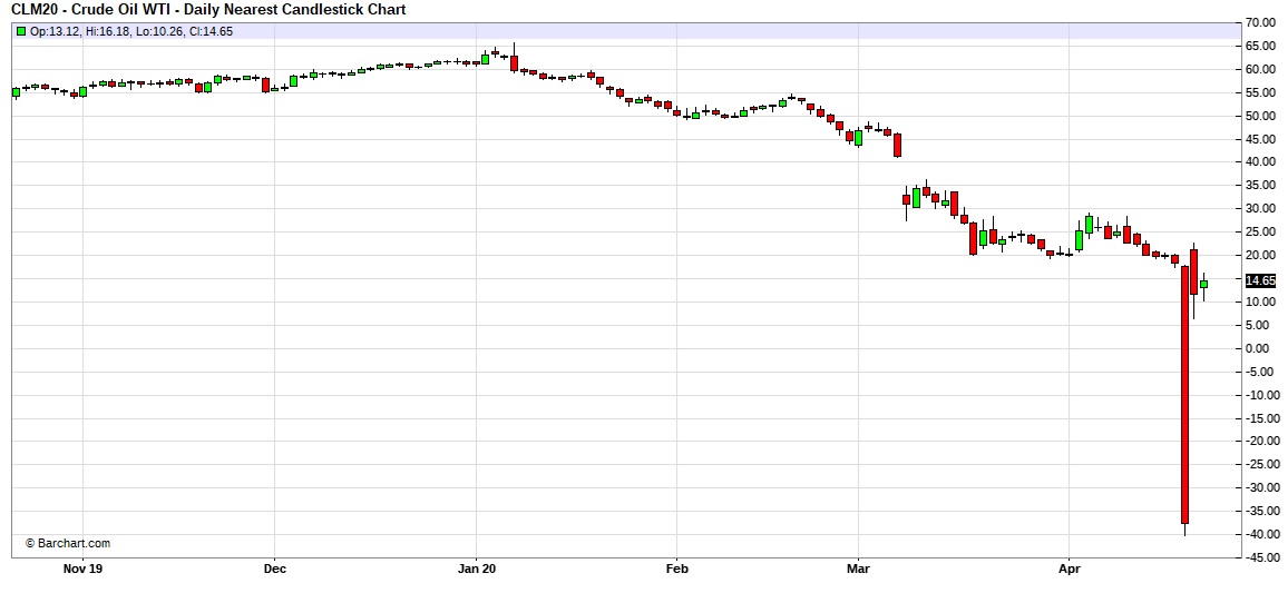
Given the remarkable events of the past week, we are adjusting the usual format of this report. We[1] have been covering energy for over three decades and never imagined that we would see prices for actively traded futures fall into negative territory.
(Source: Barchart.com)
The sharp drop in prices was mostly due to forced selling by exchange-traded products (ETPs).[2] As a reminder, there are no grantor trusts in oil, which would require the trust to hold actual barrels of oil; instead, oil ETPs usually create their products in the futures markets. Although there are various methodologies in operation, they all work, to a greater or lesser degree, by rolling contracts in different oil futures months. The most commonly used ETPs normally operate by holding the front month contract and, at some point near expiration, “rolling” into the next month. This gives an approximate constant long position in crude oil. The total return on these products come from three sources—the price of oil itself, the interest on margin,[3] and the “roll yield.” If the calendar curve for oil prices is backward (that is, the nearby futures trade at a premium to the deferred contracts), there is a positive roll yield. At each roll, under these conditions, the ETP will be purchasing a cheaper contract. If nothing changes, the cheaper contract will rise in value and benefit the ETP holder. The opposite condition, where the nearby futures trade at a discount to the deferred futures contracts, is known as contango. That is the current situation in the oil market. In this case, there would be a negative roll yield. Contango usually occurs when there is too much prompt supply relative to demand.
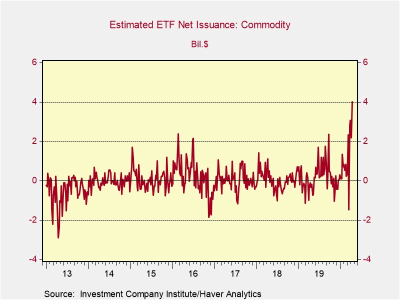
There have been reports of strong inflows into oil ETPs. Although we don’t have a breakdown by commodity, there has been a clear surge in flows. The chart below shows ETF net issuance for commodity ETPs on a weekly basis. The recent surge is notable and market commentary would suggest the lion’s share of these flows were likely into oil ETPs.
It is likely that retail investors viewed low oil prices as unsustainable and wanted to establish continual long positions for the eventual turn in prices. If not for the roll yield, this would be a reasonable strategy. But the roll yield under conditions of contango increases the cost of holding the position.
As the ETPs began the roll process, where they sold their long positions in the nearby futures and bought the next deferred contract, there was a large long position that needed to be liquidated. Unfortunately, there was little place to put the oil as the ETP doesn’t take delivery of the commodity. As of April 10, nearly 70% of storage at the Cushing, OK, delivery hub for the CME crude oil contract was utilized; it is likely that much of the rest of it was already leased. The ETPs were forced to sell to buyers that required the long to “pay” them for taking the oil off their hands, leading to the historic negative price for crude oil.
Some will ask, “is this a real price?” In one sense, no. We won’t see less than free gasoline anytime soon. The 2nd or 3rd next nearby futures contract is a better reflection of what is a normal price under current conditions. On the other hand, back in our futures days,[4] we remember a squawk box conference where a futures analyst suggested a price of a commodity had become “artificial”…to which a broker responded, “the margin calls, sir, are quite real.” There was damage to some investor accounts due to this debacle, to say nothing about participants in futures that made outsized gains and losses unexpectedly; imagine how it would be if a long equity position could see the stock price fall below zero. I am not sure this will ever happen again, but the continued squeeze on storage means that at every expiration there is a chance that something like this could be repeated.[5] If it does, the CME contract is in grave danger; we could see a shift to using Brent futures, which exhibited none of this behavior because it has wider storage options, including a cash settlement. The broader issue is that oil fundamentals are abysmal and until supply contracts and demand expands, prices will remain under pressure.
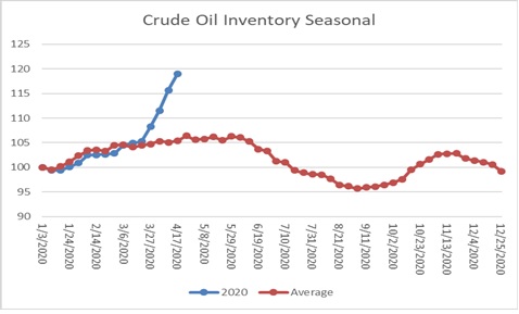
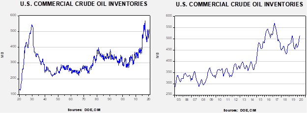
Crude oil inventories rose 15.0 mb compared to the forecast rise of 14.0 mb.
In the details, U.S. crude oil production fell 0.1 mbpd to 12.2 mbpd. Exports fell 0.5 mbpd, while imports declined 0.7 mbpd. Refining activity fell 1.5%, a bit less than the 2.0% decline forecast. The inventory build was mostly due to the continued collapse in refinery operations.
(Sources: DOE, CIM)
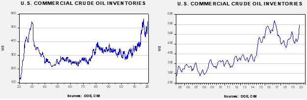
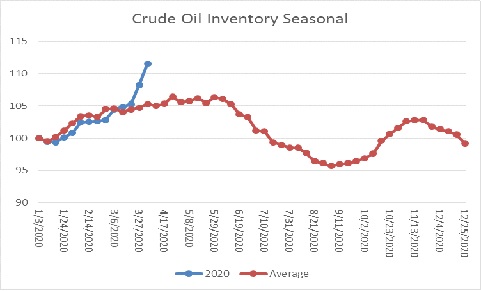
The above chart shows the annual seasonal pattern for crude oil inventories. The last four weeks have pushed stockpiles almost “off the charts.” Although not totally unexpected, the divergence in seasonal patterns could diverge in a bearish fashion in early June.
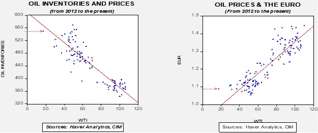
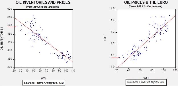
Based on our oil inventory/price model, fair value is $33.63; using the euro/price model, fair value is $44.77. The combined model, a broader analysis of the oil price, generates a fair value of $38.70. As we noted recently, the model output is less relevant as there is a non-linearity tied to the loss of storage capacity that cannot be fully captured with these models, which has been clearly exhibited over the past week.
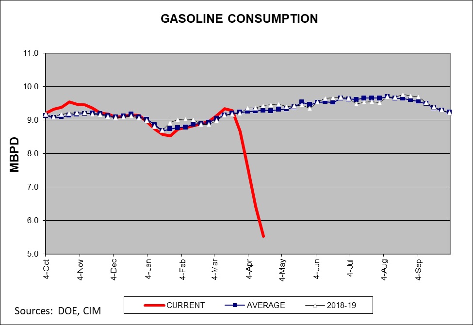
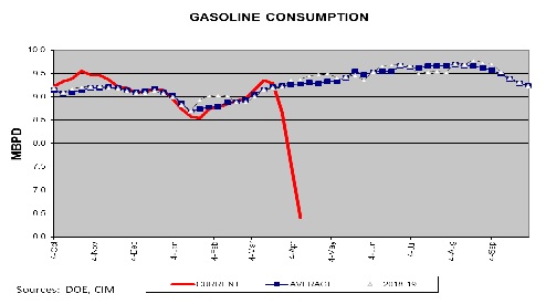
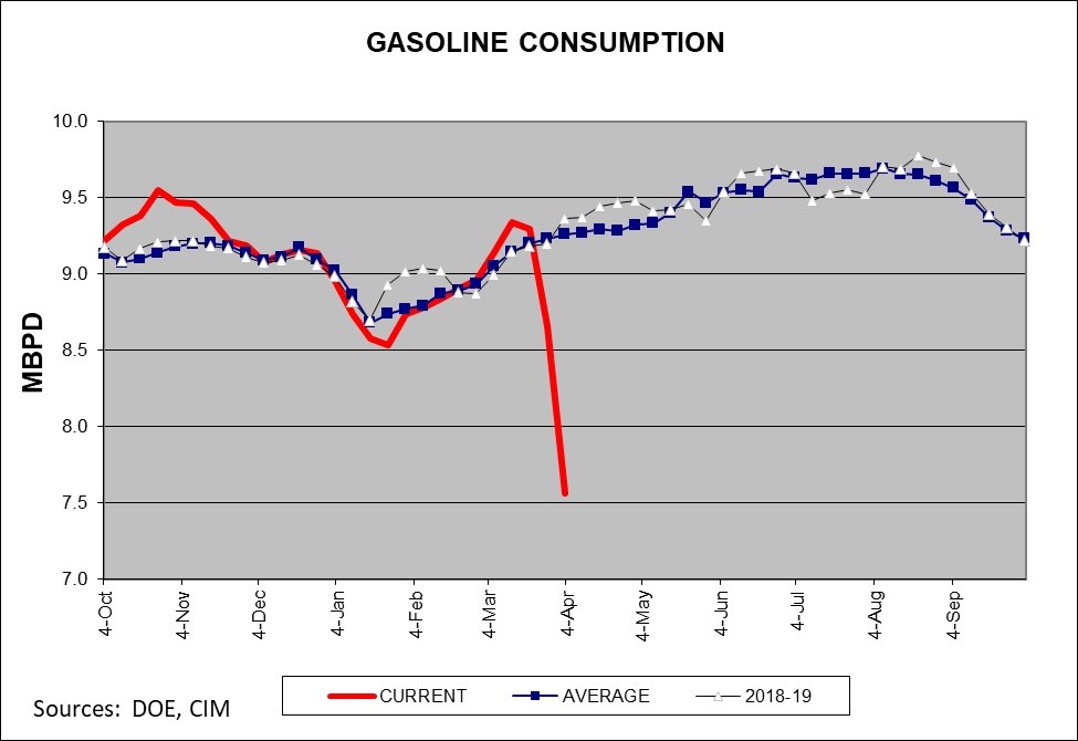
As promised, here are a couple charts that look at U.S. oil demand. The chart below shows the four-week average of gasoline supplied to the distribution system. The combination of rising inventories and lower demand has pushed up the current days to cover to nearly 48 days; the average is 25 days.
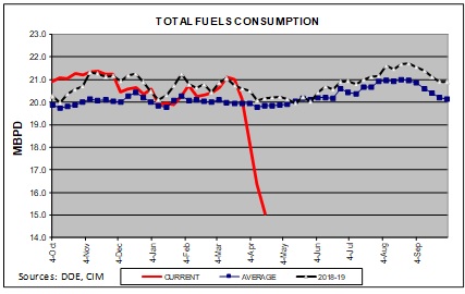
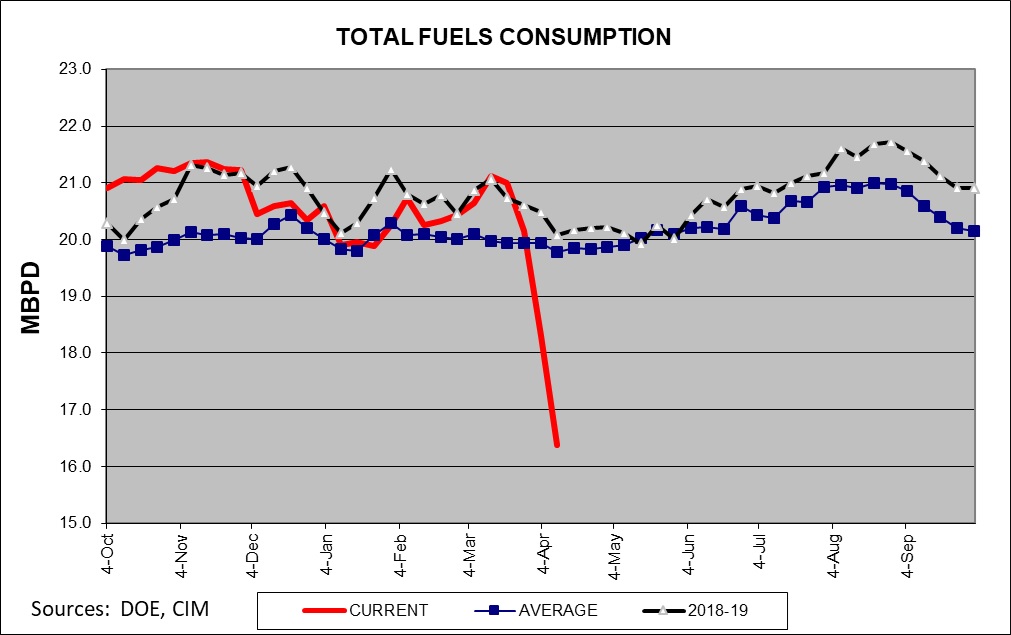
Total fuel consumption is plunging.
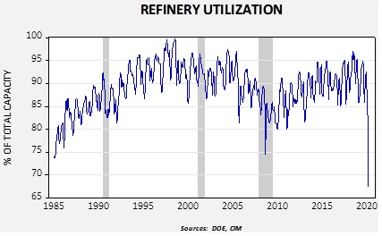
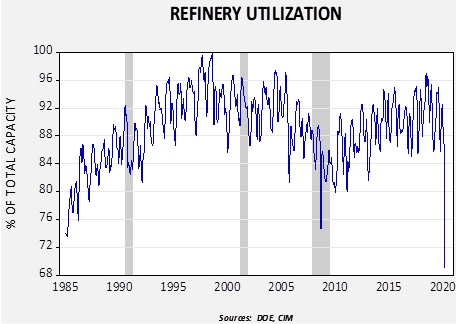
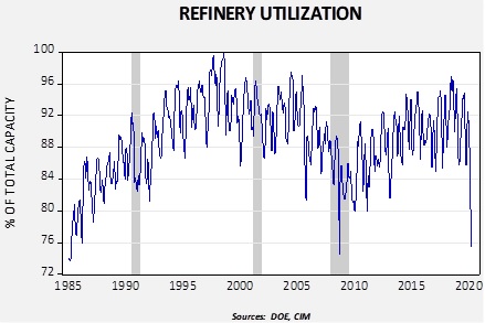
This is a longer-term view of refinery activity.
The last time we saw a drop of this magnitude was during the depths of the Great Financial Crisis. Over the past four weeks, refineries have reduced their oil consumption by 3.4 mbpd, far exceeding the drop of 0.6 mbpd in production.
So, now that oil prices have fallen precipitously, what happens now? There is a good chance that prices stay low for a rather long time. The market is building a major supply overhang that will take a long time to remove. This supply problem is being exacerbated by collapsing demand caused by the policies to reduce the spread of COVID-19. Thus, barring some event that reduces supply or boosts demand quickly, oil prices will likely languish at least into late summer. What sort of events could support a recovery in prices?
A geopolitical event in the Middle East. The potential for a disruption in oil flows is always possible. Lately, Iran has become more aggressive in harassing shipping in the Persian Gulf. The White House has warned Iran about this behavior. We doubt Iran wants a full-scale conflict with the U.S., and we doubt the U.S. wants a war either. There is the potential that both parties could stumble into a conflict, but it isn’t likely and would not be a reason to buy oil at this point.
Governments could absorb some of the overhang for strategic reserves. Such purchases would make sense. Oil prices are unusually cheap and buying emergency storage under such conditions is ideal. Australia has announced a plan to buy oil and store it in the U.S. Strategic Petroleum Reserve (SPR). It plans to purchase AUD 94.0 mm ($59 mm), roughly four million barrels of oil (at WTI $15 per barrel). China has announced purchases as well, although the actual level of injections into strategic reserves is unknown. The Trump administration has suggested SPR purchases but hasn’t been able to convince Congress to allocate funding. By itself, these purchases would not probably spark a recovery, but the buying would help.
Governments could take more aggressive actions to reduce supply. In addition to the government taking direct ownership stakes in oil companies to keep them afloat, there are reports that the administration is considering buying oil reserves from producers and simply not developing the purchased reserves, selling them at a later date when prices have recovered. This action would give cash-strapped producers cash for those assets and, at the same time, reduce future supply. There is no doubt energy-producing regions of the U.S. could use the relief. However, this plan is fraught with risk. It is not hard to imagine that a future administration could have a different policy on oil production and simply never sell or develop the purchased reserves. At the same time, this policy could have the same issues as adding oil to the SPR; it works in the short run but fashioning a policy to sell the reserves or sell oil out of the SPR has never really been done. Nevertheless, there is a chance that radical action may be taken.
Liquidate. Deep recessions and depressions reveal who is a marginal producer and who has staying power. Strong firms would likely prefer a wave of bankruptcies that would allow them to acquire assets cheaply. The fact that there is opposition to support from the oil industry suggests this sentiment remains strong. It would probably last until the strongest producers face bankruptcy; then support would be broadly welcomed. To some extent, this is the other side of the aggressive government action.
Overall, we have probably seen the lows in oil prices. It may be a few months before we see prices improve. The key factor for recovery will be a significant recovery in economic activity, which will likely come by autumn. Until then, prices will likely range in the teens into the summer.
[1] Of course, this is Bill “talking” in the royal sense.
[2] This term encompasses exchange-traded funds, exchange-traded notes and grantor trusts.
[3]Margin on June futures is $6,400 per contract. There are 1k barrels per contract, and so, at $20 per barrel, the total value of a futures contract is $20k. The ETP fully funds the contract but is only required to maintain the margin. The rest is usually held in T-bills which generate some interest income.
Today I write this quarterly client letter in the midst of a recession, one that three months ago I did not see coming. As noted in our January letter (and even italicized): We cannot predict the future. I suspect we have proved that by now. Successful long-term investing does not depend on successful forecasts of the future (which is impossible), but on accurate analyses of the present (which is possible). What we have before us, as described by Jim Bullard, president of the St. Louis Federal Reserve Bank, is a government-induced recession. Why would the government induce a recession? Don’t governments obsess over preventing recessions? Democratic governments must face the voters every few years. Recessions don’t usually lead to election victories. Even autocratic governments worry about legitimacy and the potential for revolution; they don’t want recessions either.
A government-induced recession does seem like an oxymoron, until one observes the unique threat that a highly contagious pandemic represents. Our leaders, with surprising unanimity, determined that shutting down the economy, by forcing us to shelter at home, was a preferable outcome to the potential deaths of hundreds of thousands of citizens and overwhelming the health care system. People will second-guess those decisions for generations, but that is the hand we’re dealt. We will leave it to others to assess the wisdom of policymakers’ decisions as we must invest according to the world that is, not in the world we would want.
This is a recession unlike any that we have experienced or studied. In searching for analogs, we find two other types of historical economic events to be instructive. The first is that of a mass-mobilization war, such as World War II. In that event, the government needed to redirect the productive power of the economy toward a purpose greater than normal business: winning a world-wide conflict. The government quite literally told American businesses to stop what they were doing and do something else. Auto manufacturers were told to stop making cars and trucks and start making tanks, troop carriers, and even airplanes. Consumers were told to stop normal behavior. “Stop buying tires and silk stockings, the government needs the rubber and silk; stop your usual jobs, join the military or go to work producing military equipment.” Normal economic activity was stopped by the government, while new economic activity (of the military kind) was created by the government.
Now imagine what would happen if the government told us to stop normal economic activity, but then didn’t create any new economic activity to replace it. That is what we have lived with for about five weeks in late February through late March. Government instructions to combat the coronavirus halted economic activity, but we didn’t get any action from the government to “fill the gap” until March 24. That is why the market fell 35% over the preceding five weeks (basis the S&P 500). (In fairness, one arm of the government, the Federal Reserve, has provided extraordinarily positive support to the financial system. We give them an A+.) Since then, the government has made several sizeable actions to fill the gap, and the stock market has responded positively. I’ve taken many questions about the market in the last few months, and my response has been largely the same: a cyclical low and recovery in the market will require two things – a peaking of infections and a massive response from the government to support the economy.
Mistakes by policymakers have been made and will be made. This is normal. The market will respond, not so much to the mistakes but to the effort. Since this recession was largely induced by government action (a reaction to the pandemic), honest and substantial efforts by the government to support the economy will be appreciated by investors. Thus, I believe it’s probable that the March 23 low in the market will hold. As an older (and wiser) friend and market analyst once told me, the stock market will always bottom at the point of maximum fear. On that fourth Monday in March, we were staring at an exploding health crisis while Congress dithered. Fear maxed out. When Congress got its act together in the next 24 hours, fear abated. That 35% decline in stock prices over five weeks was the fastest such decline on record, but the size of the sell-off was typical for a recession. We still can’t predict the future, but if progress is made going forward against the coronavirus and the government doesn’t ignore the economy, then we should work our way back.
I mentioned above that this unique recession is analogous to two historical economic events. In addition to a mass-mobilization war, this event is reminiscent of the effects of a natural disaster, such as a major hurricane or tornado. The difference is that a hurricane is regional, while this disaster is global. Hurricanes are devastating to the regions affected, but they have a conclusion, after which reconstruction begins. While this crisis doesn’t have the crisp endpoint of a weather disaster, it will end. And when it does end, we expect the American people will quickly go back to work to repair the damage just like they do after a tornado. Such relief and recovery usually require government assistance and support, and this disaster will be no different. But anyone who has seen a community rebuild after a hurricane or tornado has been impressed by the American spirit, and by how quickly the effects of the disaster are erased. I don’t doubt that the recovery from this disaster will be similarly impressive.
We appreciate your confidence in us.
Gratefully,
Mark A. Keller, CFA CEO and Chief Investment Officer
Although we do cover current events in the Weekly Geopolitical Report, we also try to anticipate changes that may be a consequence of current situations. The COVID-19 crisis is just such an occasion. We regularly update the current path of the virus in our Daily Comment, but we will consider the longer-term ramifications of COVID-19 in this report. We have recently discussed the pandemic, in general, in our weekly reports, and in the previous two installments we discussed how the virus has frayed relations in the EU.
This week, we frame the impact of the pandemic using Walter Scheidel’s book on inequality, The Great Leveler: Violence and the History of Inequality from the Stone Age to the Twenty-First Century.[1]We reviewed this book in a previous WGR published in 2017. In Part I, we will examine Scheidel’s thesis that says inequality tends to be resolved by violent or extreme events. Simply put, history shows little evidence that periods of high inequality are reversed without tragedy. Using this thesis, we will examine how the COVID-19 pandemic best fits into Scheidel’s framework. In Part II, we will discuss the equality/efficiency cycle and introduce one of five problems that could be resolved by the pandemic. In Part III, we will examine the other four problems, discuss the impact of inflation and conclude with market ramifications.
[1] Scheidel, Walter. (2017). The Great Leveler: Violence and the History of Inequality from the Stone Age to the Twenty-First Century. Princeton, NJ: Princeton University Press.
The Federal Reserve’s aggressive expansion of its balance sheet has been in response to fears of systemic risk. The experience of the 2008 Great Financial Crisis has made it clear that systemic risk can occur from a myriad of different parts of the financial system, so the Fed has broadened its support to include a significant expansion of credit risk, including corporate credit, both investment-grade and below-investment-grade, municipal debt, commercial paper along with mortgage and Treasuries. Although the Fed did similar actions in the depths of the 2008 Great Financial Crisis, the current policy actions are far more aggressive than what was seen in the last decade, both in the level of the balance sheet expansion and the breadth of assets being purchased. The Fed’s balance sheet is currently $6.083 trillion, a new record high.
Although the FOMC’s actions have been in response to concerns over systemic risk, there is a structural backdrop as well. Private sector debt in the U.S. is elevated and is probably unsustainable at current levels. The sustainability of debt levels is more art than science. Although there are obvious ways to measure debt service costs and one can compare historical levels, there is a psychological element to the lending and borrowing process. If confidence is high, lenders are anxious to “put money to work” and borrowers have high hopes that their borrowing will be beneficial. For example, Americans believed that home prices would continue to rise from 1995 to 2005 and lending that now looks reckless seemed reasonable at the time. But, once confidence in home prices waned, there was a scramble to reduce exposure to the sector that culminated in the 2008 Great Financial Crisis.
We have seen a decline in private sector debt[1] since 2007; however, the slow growth seen during this expansion likely reflects the fact that we haven’t seen enough debt liquidation. We saw a similar situation in the 1930s.
When private sector debt becomes excessive, there are two paths of resolution. The first is to allow the debt to be liquidated through bankruptcy. At a microlevel, this path is perfectly reasonable. After all, if a borrower and a lender took risks, they should bear the burden of their mistakes. However, at a macrolevel, this path of resolution tends to create systemic risk.[2] One party’s debt is another party’s asset. If the debt is resolved at a loss, the asset falls in value too. The process can lead to deep and widespread collateral damage. For example, in 1928 there were 26,401 commercial banks in the U.S.; by 1934, this number had declined to 15,913. The decline in asset values and the loss of bank deposits tend to lead to bank failures and the hoarding of cash that can cause a deflationary spiral. Politically, allowing a debt restructuring to occur “naturally” has become a non-starter.
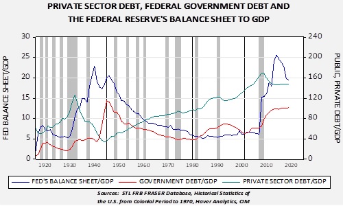
Therefore, if the private sector debt overhang isn’t resolved by liquidation and asset price declines, the other option is to socialize the debt. The debt is shifted to the public sector balance sheet and resolved over time. Referring to the above chart, the Fed’s balance sheet began to rise aggressively after 1932, with only a modest increase in the government’s debt. Although the expansion of the Fed’s balance sheet helped end the initial phase of the Great Depression, private sector debt continued to decline, which we would argue shows a continued lack of confidence by borrowers and lenders.
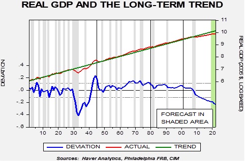
This chart shows real annual log-transformed GDP starting in 1901. We regress a time trend through the data. Despite the Fed’s efforts, GDP remained below trend, suggesting the full impact of the debt liquidation tied to the Great Depression had not been resolved. The full resolution wasn’t accomplished until the rise of government spending for WWII, along with the further expansion of the Fed’s balance sheet. The combination led to a decline in private sector debt to below 40% of GDP. The decline in private sector debt laid the groundwork for the postwar recovery. It took nearly 15 years, a massive expansion of the Fed’s balance sheet and WWII spending to fully resolve the private sector debt overhang that developed prior to the 1930s.
However, the private sector debt didn’t disappear—it was transformed into public sector debt and that debt overhang needed to be resolved. That resolution was executed by financial repression and regulation. It is important to note that government debt issued in the currency that government controls is different that private sector debt. The former doesn’t actually need to be paid off; it merely needs to be serviced. Servicing government debt is a function of the relative size of that debt to the economy. The formal process is called the Net Fiscal Effect. This process is a formula:
Net Fiscal Effect = (y/y% nominal GDP – government interest rate) + primary balance as % of GDP
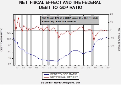
If nominal GDP rises faster than the rate of interest the government pays on the debt plus primary balance,[3] then the overall government debt/GDP ratio will fall. Here is a chart:
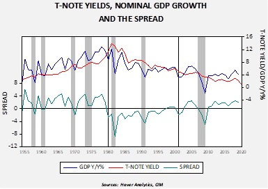
This chart shows the net fiscal effect on the upper line (we use the 10-year T-note yield as a proxy for borrowing costs). From the end of WWII into the early 1980s, the net fiscal effect was positive, and the government debt/GDP ratio steadily declined.
If policymakers follow the Great Depression/WWII path, we would expect a gradual rise in long-term interest rates.
This chart shows the 10-year T-note yield, the yearly change in nominal GDP and the difference between the two series. The postwar period to the early 1980s was a secular bear market for bonds. That may not happen this time around, or it may be slower to evolve. The Fed may engage in yield curve control, preventing Treasury rates from rising. The aging population could reduce inflation fears; it is important to note that the Millennial generation may be scarred by the last two decades and may behave like the Depression/War generation. That would mean less spending and risk taking. But it would be reasonable to expect that a gradual reflation is likely; after all, it supports the net fiscal effect.
What should investors do in this environment? We will discuss this issue at much greater length in an upcoming WGR series but here is how we are dealing with this development in our Asset Allocation strategies:
We have deployed bond ladders using ETFs. Bond laddering is an effective way to deal with gradually rising interest rates. We use a mix of corporate and Treasuries in the ladders.
We have added allocations to precious metals across all portfolios.
Historically, equities have been a good inflation hedge; however, we may see a period of adjustment in the next decade as investors deal with rising inflation. This may entail multiple contraction. Although it is too early to reduce equity exposure for this event, we are cognizant of future development.
Addressing the private sector debt overhang through socializing it to the public balance sheet is a rare event. This one will be a challenge for investors, but it can be managed. However, what has worked for the past 40 years (equity investing via blind indexing, holding long duration bonds, etc.) probably won’t work for the next four decades.
[1] We define private sector debt as household debt plus non-financial corporate debt; the financial system debt is excluded because much of that debt is to the non-financial components and thus including it would be double counting.
[3] The primary balance = government revenue/GDP – (government spending – interest paid)/GDP. In other words, it’s net government spending less interest payments.
by Bill O’Grady, Thomas Wash, and Patrick Fearon-Hernandez, CFA
Crude oil inventories rose 19.2 mb compared to the forecast rise of 11.6 mb.
In the details, U.S. crude oil production fell 0.1 mbpd to 12.3 mbpd. Exports rose 0.6 mbpd, while imports declined 0.2 mbpd. Refining activity fell 6.5%, well more than the 2.2% decline forecast. The inventory build was mostly due to the continued collapse in refinery operations.
(Sources: DOE, CIM)
The above chart shows the annual seasonal pattern for crude oil inventories. The last three weeks have pushed stockpiles almost “off the charts.” Although not totally unexpected, this is the first week where the impact of COVID-19 and the oil war have started to affect the weekly data.
Based on our oil inventory/price model, fair value is $38.75; using the euro/price model, fair value is $44.90. The combined model, a broader analysis of the oil price, generates a fair value of $41.04. As we noted recently, the model output is less relevant as there is a non-linearity tied to the loss of storage capacity that cannot be fully captured with these models. If storage capacity is fully utilized, a catastrophic decline in prices, which we would define as low teens, is possible.
As promised, here are a couple charts that look at U.S. oil demand. The chart below shows the four-week average of gasoline supplied to the distribution system. As the chart shows, shipments have cratered. Distillate demand is holding up better, reflecting the increases in delivery of goods.
Total fuel consumption is plunging.
This is a longer-term view of refinery activity.
The last time we saw a drop of this magnitude was during the depths of the Great Financial Crisis. Over the past four weeks, refineries have reduced their oil consumption by 3.2 mbpd, far exceeding the drop of 0.5 mbpd in production. The underlying fundamentals for crude oil continue to deteriorate. The DOE reduced its forecast for U.S. production this year to 11.8 mbpd. This means that production can be expected to decline further.
The Trump administration did patch together a broad OPEC+ deal; in total, the participants agreed to reduce oil output by 9.7 mbpd. However, as is usually the case with these sorts of agreements, the details tend to underwhelm. Some of the nations involved used higher baselines to make their announced cuts. Our take is that the OPEC+ cuts are probably more in the neighborhood of 7.0 mbpd. And, that relies on Russia actually cutting output, which is something of a rarity; the Russians usually promise but tend not to deliver. The OPEC+ group and the G-20 have promised production cuts of up to 20.0 mbpd. Although that cut would help stabilize the market, there is a high degree of skepticism surrounding the deal. One element of skepticism is that the KSA has cut its posted prices to Asia, while increasing them to the U.S. Part of the share war was over the Chinese market and Saudi Aramco’s (2222, SAR 30.70) decision to lower prices to the Asian market suggests the KSA isn’t really backing down. At the same time, raising the U.S. price will likely mollify the Trump administration.
Making the U.S. happy is critical to the KSA. The kingdom relies heavily on the U.S. military for protection and it needs the U.S. financial markets to recycle its dollar balances from oil. President Trump had numerous levers to pull to elicit Saudi cooperation. The U.S. could have implemented tariffs or quotas on Saudi oil imports. Military support could have been reduced. Perhaps the most potent threat would have been to deny the KSA access to U.S. financial markets. The Saudis were going to make a deal with the U.S.; the bigger issue is whether the deal will be effective.
Market conditions are better with the arrangement than without. If negotiations would have failed, it would have led to catastrophic market conditions. A plunge in prices to single digits would have been likely. Such a decline may have triggered political instability in the Middle East and triggered a corresponding spike in prices. A deal does avoid massive market volatility.
However, as the steady decline in prices this week suggests, the deal doesn’t solve the low-price problem either. That’s because we are seeing a massive drop in demand. The IEA projects that oil demand will fall by 23.1 mbpd in Q2 compared to the previous year. The proposed output cuts simply can’t offset declines of such magnitude.
Our expectation is that oil prices will fall steadily into the low teens. Markets without interference will eventually clear. They will clear by higher cost producers ceasing production. In the private sector for oil, this will mean bankruptcies and buyouts. Some production that gets shut-in probably never comes back. In Texas, some producers are calling for the Texas Railroad Commission to step into the market and allocate production, something this body did from 1932 to 1970. Companies operating in the state are divided on this action as is the commission itself. The legality is on somewhat thin ice (production allocation violates U.S. antitrust laws). Our read is that conditions will need to get much worse before there is a unified response for such action. That scenario may occur in the coming weeks.
A new solution has emerged—paying oil companies not to produce. The U.S. has a long history of intervening in commodity markets. The grain markets have deep government involvement. The USDA has bought grain from farmers at set prices, paid farmers not to grow crops on marginal fields, and simply paid farmers money (as we saw last summer due to the trade war with China). We think we are still some distance from this outcome but, for the first time, direct aid to oil companies is being considered. We will see how Congress handles that appropriation. Perhaps this could be a bargaining point for the stalled small business aid boost.
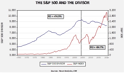
One of the more controversial issues of the past bull market was the impact of share buybacks. The way we like to frame that issue is with the S&P 500 divisor. The divisor is a number that is used to smooth out the index; when stocks leave the index, through replacement or mergers, or when new stock is issued or purchased, the divisor adjusts to prevent discrete jumps in the index. Therefore, if companies are buying back stock, the divisor will decline, all else held equal.
This chart shows the divisor and the S&P 500 from 1964. In general, it would be reasonable to assume that as stock prices rise, but especially if the P/E multiple rises, companies would generally want to issue stock. Thus, the divisor would be expected to follow the overall movement of the market. And, from 1964 until 2004, that was generally true. The two series were positively correlated at the 74.9% level. However, from 2005 to the present, despite a major bull market from 2009 to 2020, the trend in the divisor was lower. In fact, the sign of the correlation reversed to negative.
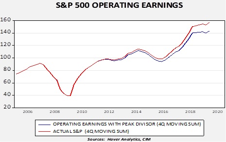
The divisor is used to calculate earnings per share; a falling divisor boosts the earnings per share reading. If we assume that the divisor had remained at the most recent peak in 2011, the chart below shows the impact on earnings per share.
This chart shows operating earnings on a rolling four-quarter basis. Using Q4 2019, the latest actual data available,[1] the reported operating earnings per share was $157.12; adjusting for the 2011 peak divisor shows a reading of $143.28.
The extensive policy actions taken by the government and the Federal Reserve to backstop the economy and the financial markets will likely come with the costs of direct regulations and social control. In other words, taking the government’s money or using the Fed’s balance sheet to simply support shareholders through dividends and buybacks is probably not going to be possible. If that is the case, it is highly likely that earnings growth will be less than what we have seen in recent years. Margins are another element we are monitoring; these have been remarkably strong for the past decade. So far, we have not seen aggressive actions to reduce margins but a retreat from globalization and a return to regulation could bring down margins as well.
[1] These numbers will appear lower than what is commonly shown because we use data from Standard and Poor’s. The media usually reports data from Thomson/Reuters, the owners of I/B/E/S, the service that collects earnings estimates. Thomson/Reuters earnings tend to be about 7% higher than Standard and Poor’s.
by Bill O’Grady, Thomas Wash, and Patrick Fearon-Hernandez, CFA
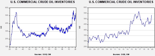
Crude oil inventories rose 15.2 mb compared to the forecast rise of 9.0 mb.
In the details, U.S. crude oil production fell 0.6 mbpd to 12.4 mbpd. Exports fell 0.3 mbpd, while imports declined 0.2 mbpd. Refining activity fell 6.7%, well more than the 1.8% decline forecast. The inventory build was due to a combination of falling exports and a severe decline in refinery operations which offset the decline in production.
(Sources: DOE, CIM)
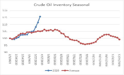
The above chart shows the annual seasonal pattern for crude oil inventories. The last two weeks have pushed stockpiles almost “off the charts.” Although not totally unexpected, this is the first week where the impact of COVID-19 and the oil war has started to affect the weekly data.
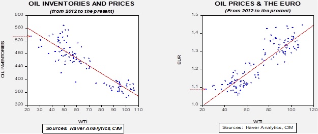
Based on our oil inventory/price model, fair value is $45.11; using the euro/price model, fair value is $44.63. The combined model, a broader analysis of the oil price, generates a fair value of $43.44. Usually, the fair value from the combined model falls within the values generated by the individual models. Recent volatility has led to some model instability, so the combined model is generating the lowest forecast price. As we noted recently, the model output is less relevant unless Russia and the Kingdom of Saudi Arabia (KSA) come to an agreement on supply. At the same time, it does show that prices in the mid-$20s have discounted a good bit of bad news. However, there is a non-linearity tied to the loss of storage capacity that cannot be fully captured with these models. If storage capacity is fully utilized, a catastrophic decline in prices, which we would define as low teens, is possible.
As promised, here are a couple of charts that look at U.S. oil demand. The chart below shows the four-week average of gasoline supplied to the distribution system. As the chart shows, shipments have cratered. Distillate demand is holding up better, reflecting the increases in delivery of goods.
This is a longer-term view of refinery activity.
The last time we saw a drop of this magnitude was during the depths of the Great Financial Crisis. Over the past two weeks, refineries have reduced their oil consumption by 2.2 mbpd, far exceeding the drop of 0.4 mbpd in production. The underlying fundamentals for crude oil continue to deteriorate. The DOE reduced its forecast for U.S. production this year to 11.8 mbpd. This means that production can be expected to decline further.
Oil prices have held up rather well because of hope of a broad deal between OPEC+others to reduce production. President Trump is threatening all sorts of actions, including tariffs and anti-dumping legislation. There is a risk to all this—such actions will raise gasoline prices over time. However, that isn’t a problem in the near term. As the above chart shows, people aren’t driving all that much. Still, we think the president doesn’t really want to directly intervene, but merely threaten Russia and the KSA into agreeing to cut output. Russia has reportedly agreed to cut 1.6 mbpd, which is boosting prices this morning.
We remain highly skeptical that a deal can be fashioned among the wide number of participants, but we would be surprised if no deal is announced. But, announcing is one thing, while actually cutting is another matter. Another point to consider—oil futures prices are running well above cash barrels as speculators hoping for a deal are buying in the futures market. At some point, these physical barrel holders are going to rush to sell their actual oil into the futures market to capture the spread. Don’t be surprised to see a “buy rumor, sell fact” trade post-agreement.
(Note: Due to the Easter holiday, our next report will be published on April 20.)
In Part I of this report we examined the history of the European Union (EU), how it works, and the political, economic, and social fissures that had already rendered it unstable when the COVID-19 pandemic took hold. This week, we look at several recent policy moves that various EU countries have taken in response to the pandemic, and we explain why those policy moves could potentially push the EU over the tipping point toward disintegration if they are carried too far. As always, we’ll wrap up with a discussion of the possible economic consequences of a break-up and the ramifications for investors.
The Temptation to Barricade
As we discussed in Part I, the founders of the EU believed that preventing another major war on European soil could be accomplished, in part, by an “ever-closer union among the peoples of Europe.” The EU is often seen mostly as an economic arrangement (i.e., a customs union coupled with a free-trade area), but its founding principles are broader than that. The EU aspires to the free movement of virtually all people, goods, services, and capital. Unfortunately, the COVID-19 pandemic has tempted EU leaders to erect barriers in these areas.
We use cookies to ensure that we give you the best experience on our website. If you continue to use this site we will assume that you are happy with it.