

Author: Rebekah Stovall
Asset Allocation Weekly (June 26, 2020)
by Asset Allocation Committee
(N.B. Due to the Independence Day holiday, the next report will be issued on July 10, 2020.)
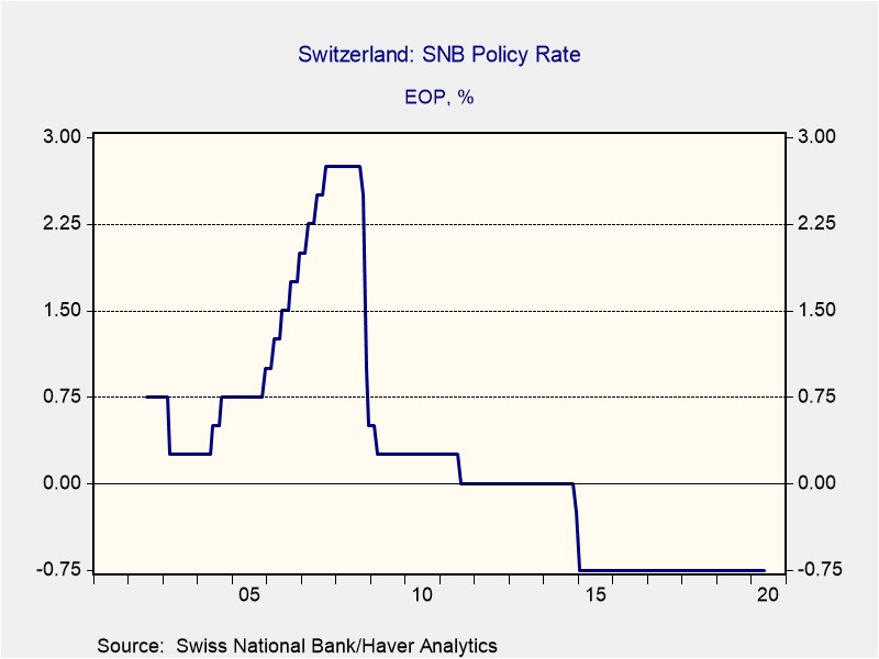
Since 2008, some central banks have implemented negative policy interest rates. Standard economics suggests that negative nominal rates on deposits are impossible because holders could simply liquidate the deposit and “put the money under the mattress.” We have observed that there are costs to holding cash in large amounts, so banks can implement a negative rate (perhaps best thought of as a fee) on holding cash. Although there are limits to how low negative rates can go (at some point, the cost of providing safekeeping exceeds the benefits), we note the Swiss National Bank has had a policy rate of -0.75% since December 2014.
Why would a central bank consider implementing a negative policy rate? If economic conditions warranted easing and inflation was low,[1] it may be impossible to use low but positive interest rates as a policy tool. In that case, negative interest rates or some other unconventional monetary policy may be necessary.
Are conditions similar in the U.S.? Our analysis of the policy rate, using the Mankiw Rule, a variation on the Taylor Rule, suggests that the FOMC could consider negative policy rates. The Taylor Rule is designed to calculate the neutral policy rate given core inflation and the measure of slack in the economy. John Taylor measured slack using the difference between actual GDP and potential GDP. The Taylor Rule assumes that the Fed should have an inflation target in its policy and should try to generate enough economic activity to maintain an economy near full utilization. The rule will generate an estimate of the neutral policy rate; in theory, if the current fed funds target is below the calculated rate, the central bank should raise rates. Greg Mankiw, a former chair of the Council of Economic Advisors in the Bush White House and current Harvard professor, developed a similar measure that substitutes the unemployment rate for the difficult-to-observe potential GDP measure. We have taken the original Mankiw Rule and created three other variations. Specifically, our models use core CPI and either the unemployment rate, the employment/population ratio, involuntary part-time employment or yearly wage growth for non-supervisory workers. In this report, we are not using the wage growth variation because it is yielding a sharply positive policy rate; wages have increased because lower paid workers have been laid off in greater numbers than higher paid workers.
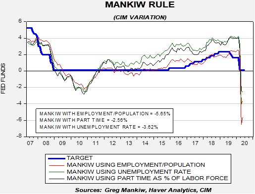
As the recession developed, the unemployment rate jumped, the employment/population ratio fell, and the number of involuntary part-time workers rose. Complicating matters further, inflation declined. All these factors pointed to the need for policy stimulus. In fact, in the worst case, the employment/ population ratio variation, the nominal rate should be as low as -5.65%.
In 2008 through most of 2011, these variations of the Mankiw Rule suggested the policy rate should have been below zero. That is the case today. So far, the FOMC has rejected a negative policy rate and instead relies on expanding the balance sheet and forward guidance. The current program of balance sheet expansion is historically unique; for the first time, we are seeing the Fed buy an assortment of financial assets that expose it to credit risk. These include corporate and high yield bonds. As we noted last week, the current QE is reducing credit spreads, but, like forward guidance, the actual stimulative impact is uncertain.
So, why is the FOMC opposed to negative interest rates? The most likely reason is the structure of the U.S. financial system. The U.S. system has an extensive non-bank financial system; unlike banks, this system isn’t funded by deposits but by repo and money markets. The non-bank financial system, also known as the “shadow banking system,” finances large swaths of the U.S. economy. Although it is difficult to estimate the size, there are reports it may be as large as $1.2 trillion. The fear is that negative deposit rates would likely cause the money market funds to “break the buck” to account for the below-zero yield. That could lead to difficult-to-determine outcomes, but it is plausible that the non-bank financial system may find itself without a source of funding. Since there is no Fed backstop to the non-bank financial system, there could be a run on the loan providers. Other nations have much smaller non-bank systems and thus can manage negative policy rates. The U.S. probably can’t.
And so, additional policy stimulus, if necessary, will come from further expansion of the balance sheet and forward guidance. Another possibility would be yield curve control, which was implemented during WWII into the early 1950s. In this policy, the Fed will set the desired rate of some or all of the Treasury curve, absorbing all the Treasury borrowing that the market won’t buy, thus fixing the interest rate. The Bank of Japan and Reserve Bank of Australia are currently running such policies. Although the FOMC hasn’t taken this step yet, it is being considered by Fed policymakers. The conclusion—monetary policy will likely remain historically accommodative well into 2021.
[1] For example, Switzerland’s May CPI was -1.3% from last year.
Business Cycle Report (June 25, 2020)
by Thomas Wash
The business cycle has a major impact on financial markets; recessions usually accompany bear markets in equities. The intention of this report is to keep our readers apprised of the potential for recession, updated on a monthly basis. Although it isn’t the final word on our views about recession, it is part of our process in signaling the potential for a downturn.
In May, the diffusion index fell deeper into recession territory as improvements in several indicators could not outweigh the negative impact of the previous two months. Last month, states started reopening their economies which resulted in a rise in economic conditions. The financial market continued to show signs of improvement as the Federal Reserve offered reassurances that it would continue to intervene in markets when needed. Additionally, increased economic activity led to a sharp rise in equities. Meanwhile, a reduction in lockdown restrictions allowed firms to hire workers in record numbers. However, the impact of the pandemic continued to weigh heavily on both investor and consumer confidence as concerns persist surrounding economic outlook. As a result, six out of the 11 indicators are in contraction territory. The reading for this month fell to -0.152 from +0.030 in April, well below the recession signal of +0.250.
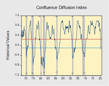
The chart above shows the Confluence Diffusion Index. It uses a three-month moving average of 11 leading indicators to track the state of the business cycle. The red line signals when the business cycle is headed toward a contraction, while the blue line signals when the business cycle is headed toward a recovery. On average, the diffusion index is currently providing about six months of lead time for a contraction and five months of lead time for a recovery. Continue reading for a more in-depth understanding of how the indicators are performing and refer to our Glossary of Charts at the back of this report for a description of each chart and what it measures. A chart title listed in red indicates that indicator is signaling recession.
Weekly Energy Update (June 25, 2020)
by Bill O’Grady, Thomas Wash, and Patrick Fearon-Hernandez, CFA
(NB: Due to the upcoming Independence Day holiday, the next report will be published on July 9.)
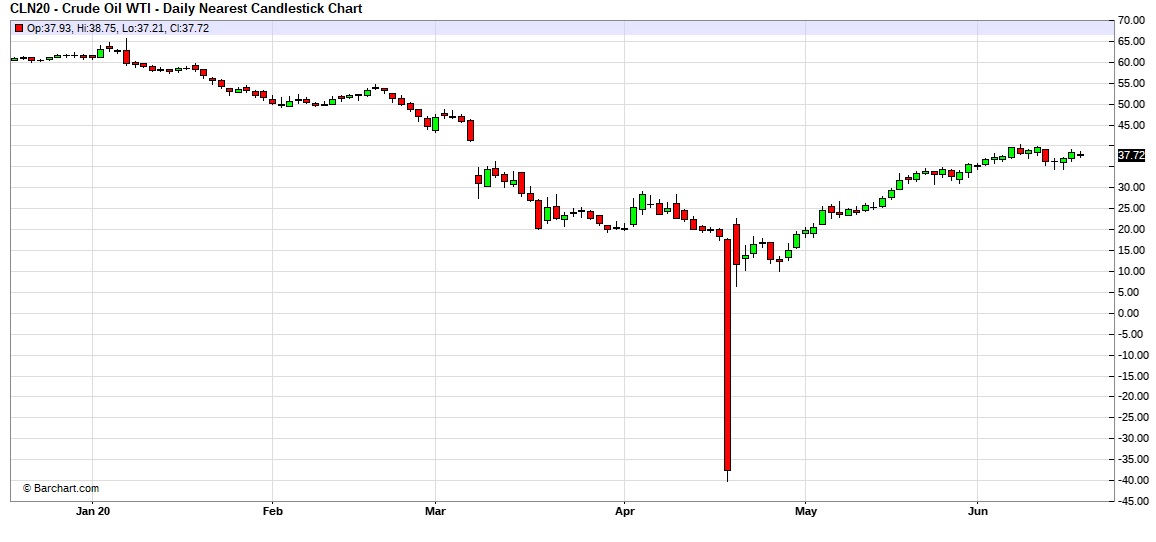
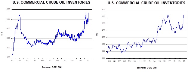
Here is an updated crude oil price chart. The oil market has stabilized at higher levels after April’s historic collapse.
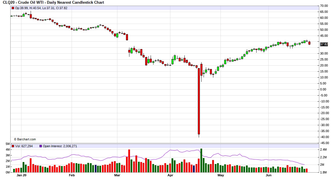
Crude oil inventories rose less than market expectations, with stockpiles rising 1.4 mb compared to forecasts of a +2.0 mb build. The SPR added 2.0 mb this week.
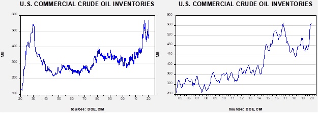
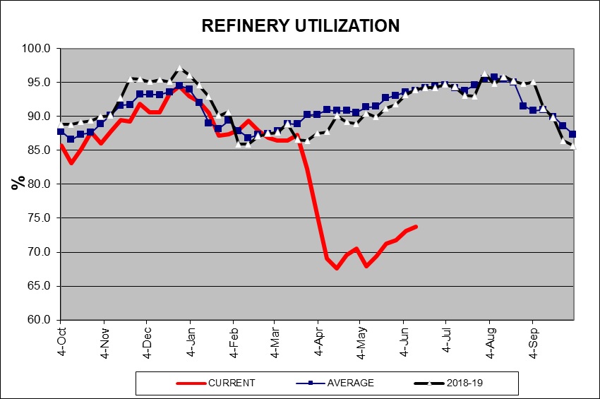
In the details, U.S. crude oil production rose 0.5 mbpd to 11.0 mbpd. Exports rose 0.7 mbpd, while imports fell 0.1 mbpd. Refining activity rose 0.8%, modestly higher than expected. After major declines for the past several weeks, the level of unaccounted-for crude oil recovered sharply this week.

Unaccounted-for crude oil is a balancing item in the weekly energy balance sheet. To make the data balance, this line item is a plug figure, but that doesn’t mean it doesn’t matter. This week’s number is -53 kbpd. This is a very small number and suggests the DOE is getting the data fixed. The rise in production suggests that the unaccounted-for crude oil data was being affected more by crude oil stored in areas unreported, although falling output addressed some of this figure as well.
We have been seeing oil flow into the Strategic Petroleum Reserve (SPR) in recent weeks. The government is offering storage in the SPR to relieve inventory constraints. The chart below shows the history of the level of inventory in the SPR by party holding the White House.
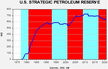
Although President Carter was an exception, in general, Republicans have tended to build the SPR, while Democrats have held it mostly steady. This may be due, in part, to the fact that the GOP tends to favor the energy industry. President Trump has not followed that pattern until recently. We do expect these injections to be temporary as the rise is due to aiding the industry and not a deliberate policy to increase the stockpile. But, since mid-April, 18.8 mb have gone into the SPR, easing bearish price pressures.
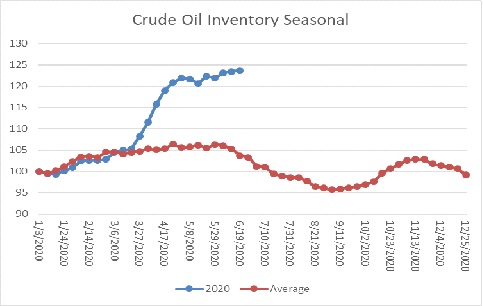
The above chart shows the annual seasonal pattern for crude oil inventories. This week’s data showed another modest rise in crude oil stockpiles. We are in the beginning of the seasonal draw for crude oil. The continued rise in inventories is bearish for prices.
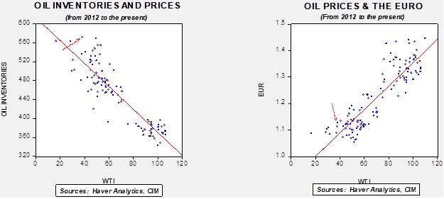
Based on our oil inventory/price model, fair value is $26.85; using the euro/price model, fair value is $52.56. The combined model, a broader analysis of the oil price, generates a fair value of $39.99. We are starting to see a wide divergence between the EUR and oil inventory models. The weakness we are seeing in the dollar, which we believe may have “legs,” is bullish for crude oil and may overcome the bearish oil inventory overhang.
Gasoline consumption remains below average, but the recovery is unmistakable.
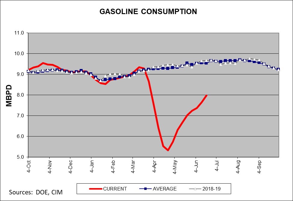
Still, the refining industry is continuing to struggle, and without improvement in this sector the demand for crude oil could stall in the coming weeks.
Confluence of Ideas – #13 “The 2020 Election: Part 1” (Posted 6/23/20)
Weekly Geopolitical Report – The Geopolitics of the 2020 Election: Part V (June 22, 2020)
by Bill O’Grady | PDF
This is the final report in our five-part series on the geopolitics of the 2020 election, which was divided into nine sections. This week, we conclude the report by covering the eighth and ninth sections, the base cases for a Trump or Biden win and market ramifications.
Asset Allocation Weekly (June 19, 2020)
by Asset Allocation Committee
By now, investors have rightly come around to the idea that the equity market’s strong rebound since late March can be largely ascribed to the aggressive monetary and fiscal policies put in place to counter the coronavirus crisis. The economic downturn from the pandemic lockdown has been severe, pushing unemployment to its highest level since the Great Depression and freezing demand for most products. All the same, the Federal Reserve’s massive bond-buying and the federal government’s gigantic spending programs have convinced many people that the public sector is doing what’s necessary to support a quick recovery and minimize the long-term damage. Investors have bid up stocks in response. The technology-heavy NASDAQ has even reached a new record high.
What’s gotten less attention is that the policy moves have also helped limit the damage in the debt markets. That’s especially clear in the market for riskier debt that the credit rating firms consider to be below-investment grade, i.e., “high yield” or “junk” bonds. One way to measure the demand for that kind of debt is to compare the yield investors are requiring for that kind of bond versus the yield on a risk-free bond of similar maturity, such as the five-year Treasury note. As shown in the chart below, the effective yield on the BofA Merrill Lynch High-Yield Master II Index spiked to as much as 8.57% at the peak of the coronavirus crisis in March and April. At the same time, safe-haven buying drove down the yield on the five-year Treasury note to just 0.39%. That boosted the high-yield spread over the five-year Treasury all the way to 8.18% compared with an average spread of 5.61% over the last several decades.
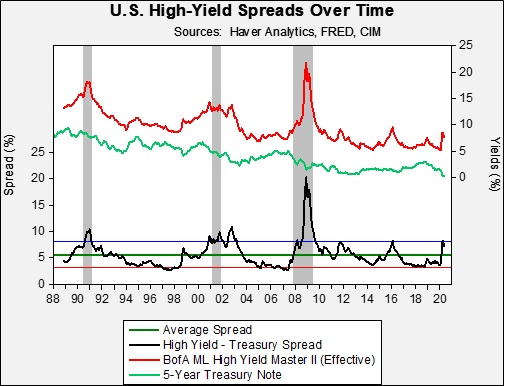
As shown in the chart, the April spread of 8.18% was one full standard deviation above the average spread since 1988. But instead of rising even further above the one-standard deviation mark as typically happens during a recession, the spread has fallen modestly in May and June. We think that’s a clear indication that investor nerves have been calmed by the aggressive monetary and fiscal policy already put into place. One particularly helpful move was the Fed’s decision to purchase corporate debt, ultimately including debt that had been downgraded to junk status after March 22 and corporate bond ETFs that might hold high-yield obligations.
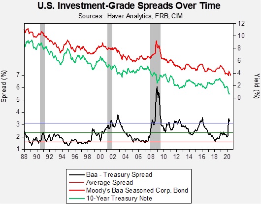
By pumping liquidity into the economy and helping many firms avoid bankruptcy, the U.S. policy moves have helped bolster not only junk bonds, but also investment-grade bonds and equities. For example, the chart below shows how the spread of corporate investment-grade yields over the 10-year Treasury also initially spiked and then narrowed after the policy moves were implemented. The pattern looks very similar to the narrowing of high-yield spreads. Although the financial markets remain volatile and credit spreads could widen again, we think the early signs of credit spread narrowing support increasing exposure to corporate credit in portfolios.
Weekly Energy Update (June 18, 2020)
by Bill O’Grady, Thomas Wash, and Patrick Fearon-Hernandez, CFA
Here is an updated crude oil price chart. The oil market has stabilized at higher levels after April’s historic collapse.
Crude oil inventories were mostly in line with market expectations, with stockpiles rising 1.2 mb compared to forecasts of a 0.8 mb draw. The SPR added 1.7 mb this week.
In the details, U.S. crude oil production fell 0.6 mbpd to 10.5 mbpd. Exports were unchanged, while imports fell 0.2 mbpd. Refining activity rose 0.7%, in line with expectations. As we have seen in recent weeks, the level of unaccounted-for crude oil remains elevated but did decline this week.
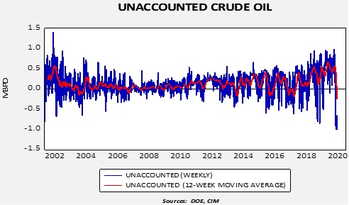
Unaccounted-for crude oil is a balancing item in the weekly energy balance sheet. To make the data balance, this line item is a plug figure, but that doesn’t mean it doesn’t matter. This week’s number is -0.7 mbpd. The fact that the decline fell from 1.0 mbpd to 0.7 mbpd and coincided with a sharp drop in oil production suggests that this number is reflecting falling output. Simply put, oil production is falling faster than the official data suggest.
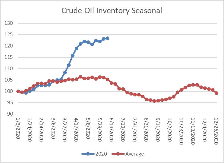
The above chart shows the annual seasonal pattern for crude oil inventories. This week’s data showed a modest rise in crude oil stockpiles. We are on the cusp of the beginning of the seasonal draw for crude oil. If inventories don’t decline in the coming weeks, oil prices would be vulnerable to a correction.
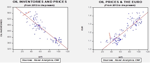
Based on our oil inventory/price model, fair value is $27.27; using the euro/price model, fair value is $52.74. The combined model, a broader analysis of the oil price, generates a fair value of $40.24. We are starting to see a wide divergence between the EUR and oil inventory models. The weakness we are seeing in the dollar, which we believe may have “legs,” is bullish for crude oil and may overcome the bearish oil inventory overhang.
Although conditions in energy are improving, the recovery is slow. Refining operations are 20 points below average.
The IEA forecast a sharp recovery in oil demand in 2021, which we would expect. This year’s crude demand is expected to fall 8.1 mbpd but rise 5.7 mbpd next year.
Weekly Geopolitical Report – The Geopolitics of the 2020 Election: Part IV (June 15, 2020)
by Bill O’Grady | PDF
In this five-part series on the geopolitics of the 2020 election, we have divided the reports into nine sections. Last week, in Part III, we covered the incidence of establishment policy and the role of social media. This week, we reveal the sixth and seventh sections; we handicap the race as it stands and discuss how foreign nations are likely to intervene in the election.
Who is Going to Win?
Before we discuss our expectations of the outcome, we want to note that we analyze elections with an eye toward answering two questions. First, who is going to win? Second, what will they do once elected? In our primary role of managing money, we cannot afford to allow any political preference to distort our process as that bias could affect investment performance. And, being well ensconced in the flyover zone of the U.S., our political biases don’t matter anyway. It’s not as if our analysis affects the actual outcomes of elections. Our position is that, as a money manager, we want to know what the future looks like, not necessarily root for a certain outcome. So, here goes.
To forecast the outcome of elections, we have various factors we examine that have signaled the outcomes of previous elections. These factors are:
- Incumbency
- The Economy
- Polling
- Prediction Markets
- Base of Support
- Money
- Social Media Presence
We are also sensitive to the fact that we don’t directly elect presidents; we elect electors to the Electoral College who, in most states, vote for the president based on the majority of votes in that state.[1] So, our focus is on determining our best estimate of the Electoral College based on polls and available decision markets, along with economic activity at the state level.