After a short foray into emerging markets, we exited that position in our latest allocation. Prior to the Trump victory, we had expected the dollar to weaken which would have supported emerging markets. However, the dollar’s resurgence is a bearish factor for emerging markets, leading the Asset Allocation Committee to look elsewhere for return.
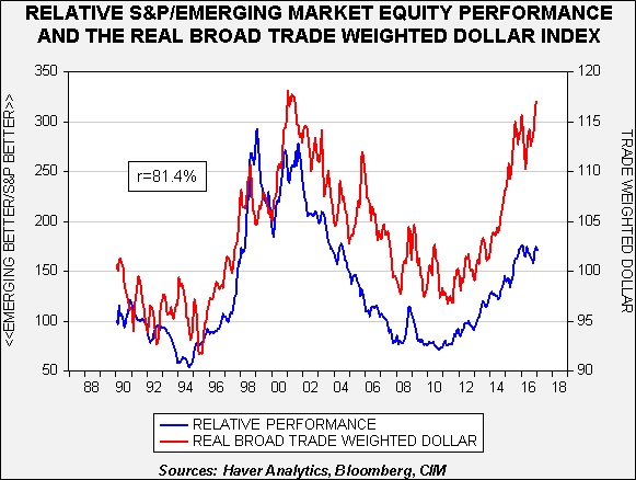
The blue line on this chart looks at the relative performance of emerging markets to the S&P 500. When the line is rising, the S&P is outperforming emerging markets. The red line is the JPM real dollar index. The two series are positively correlated at 81.4%, meaning that a stronger dollar tends to support the S&P relative to emerging markets.
Although the dollar is richly valued based on most currency valuation models, we believe that two factors will tend to support continued strength.
The Federal Reserve is set to accelerate its rate hikes this year, while other major central banks are looking to maintain stimulus. Although the stronger dollar may slow the pace of tightening, comments from the FOMC suggest a wide variation of opinions on the impact of the dollar on the economy. Thus, until it is abundantly clear that the exchange rate is hurting the economy and lowering inflation, we suspect the Fed will move rates higher.
Fiscal and trade policy are being designed to reduce imports. President-elect Trump is publically shaming firms for investing outside the U.S. and threatening trade restrictions against countries like China. Speaker Ryan’s corporate tax reform includes a “border adjustment” that would effectively tax imports and not tax exports. When the reserve currency nation restricts trade, it reduces the supply available to world markets. Since there is no clear substitute for the dollar for reserve purposes, meaning the slope of the demand curve should remain static, a drop in supply should lead to a stronger dollar.
Eventually, the dollar will rise to a level that will fully offset the impact of relatively tighter monetary policy and changes in fiscal and trade policy. Although an exact level is difficult to determine, we would expect the JPM dollar index to rise to levels of past bull markets.
To reach levels seen in the 1995-2001 bull market, the dollar index should rise about another 10%. We doubt we will reach the highs of the Volcker dollar bull market (which would entail another 20% increase from current levels), but we would not be surprised to see a level between the two bull phases. Such a rise will pressure emerging market equities.
Finally, it is worth noting that the 1982 Mexican Debt Default and the 1997-99 Asian Economic Crisis occurred during rising dollar markets. Dollar strength tends to weigh on commodity prices, which often are produced by emerging market nations. In addition, emerging market nations and companies often borrow in dollars at lower interest rates relative to domestic rates. A rising dollar raises debt service costs and increases the odds of default.
Thus, for the time being, we intend to forego a position in emerging markets. However, once the dollar bull market is exhausted, emerging market equities could become attractive.
Last week, we reviewed Sebastian Mallaby’s recent biography of Alan Greenspan.[1] This week, we will focus on the issue of financial crises and financial stability. As noted in last week’s review, the financial system has evolved from a disjointed and diffuse system where banks could not establish themselves across state lines to one of increasing interconnectedness and concentration. Although this has made the financial system more efficient, it has also made it less robust. Simply put, we have created a “too big to fail” problem that means that the Federal Reserve must stand ready to intervene and support failed financial firms to prevent a broader systemic meltdown. This factor, coupled with inflation targeting, means that policy will tend to produce rising financial asset markets that are prone to infrequent large bear markets. The analogy we have used in the past is similar to a forestry policy that will not tolerate any forest fires. By preventing small fires, excessive underbrush grows, creating conditions that allow for extreme fire events that are difficult to control. By constantly rescuing smaller financial firms, policymakers encourage excessive risk which leads to unstable financial markets.
If FOMC officials are convinced that regulators and financial policymakers will not address the “too big to fail” issue effectively (and we tend to believe they won’t[2]), then in reality the Federal Reserve has three mandates—full employment, controlled inflation and financial stability. Currently, the FOMC uses monetary policy to address the first two mandates and relies on regulation to manage financial stability. The track record for regulation is poor—even Vice Chair Fischer noted that so called “macro-prudential regulations” don’t work all that well, based off his experience as head of the Bank of Israel.[3] Regulatory capture, the phenomenon where regulators are co-opted by those they regulate, is well-documented. The only effective policy available to manage financial stability is monetary policy—raising or lowering interest rates. However, it is very difficult for a central banker to raise interest rates because the equity P/E is too high or bond yields are too low; in fact, as we noted last week, it’s a good way for a central bank to see its independence stripped.
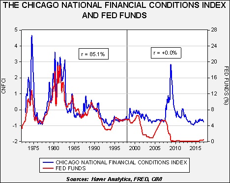
We have previously discussed the disconnect that has developed between financial stress and monetary policy.
This chart shows the Chicago FRB’s Financial Conditions Index (“CFRBFCI”) and the rate of fed funds. The CFRBFCI is a measure of financial stress—it has 105 variables that include interest rates, borrowing levels, outstanding debt, credit spreads, credit surveys and money supply among many other factors. In general, a rising number suggests worsening financial conditions and a reading above zero indicates worse than average financial conditions. From 1973, when the index was first created, until the end of 1997, the CFRBFCI and the level of fed funds were closely correlated, at +85.1%. When the Fed raised rates, financial conditions generally worsened and vice versa. Essentially, this relationship acted as a “force multiplier” for monetary policy. When the Fed raised rates, worsening financial conditions acted to depress the economy; when the Fed cut rates, improving financial conditions boosted growth. However, since 1998, the two have become completely uncorrelated. When the FOMC raised rates from 2004 to 2006, financial stress didn’t rise; when the financial crisis hit in 2008, the sharp drop in rates was slow to lower stress. In fact, it wasn’t until April 2013 before financial stress fell to pre-crisis levels.
We have puzzled over this change for some time. Mallaby’s biography of Greenspan offers one possible explanation. In 1998, during the Long-Term Capital Management meltdown and Asian Economic Crisis, the FOMC, pressed by Greenspan, cut rates 25 bps at three consecutive meetings (Sept. through Nov.). These cuts occurred in an environment of steadily falling unemployment. Simply put, the FOMC cut rates as financial stress rose even though the case for lowering rates was difficult to justify given the state of the economy. It appeared that investors concluded a policy asymmetry was in place—policymakers would cut rates if financial stress rose but would refrain from raising rates if stress was low. In other words, the “Greenspan put” on financial markets was in place.
This leads to a rather uncomfortable problem. If monetary policymakers are concerned that the financial system is fragile and cannot cope with much financial stress and they also conclude that regulators will never address this fragility due to regulatory capture, then they will be reluctant to raise rates and will only do so by clearly telegraphing their plans to avoid creating financial stress. There are four conclusions to draw from this problem. First, since the Fed will continue to target inflation, which is mostly held in check by globalization and deregulation (characterized mostly as the unfettered introduction of technological change), there will be a tendency for asset prices to reach unsustainable levels. Second, given the impotence of financial regulation, the FOMC will unofficially target the suppression of financial stress, also fostering higher financial asset prices. Third, investors will realize that the policy of suppressing financial stress will allow them to take on more risk.[4] Fourth, monetary policy will be only modestly effective in reducing financial stress when the inevitable drop in asset values eventually occurs.
For investors, this policy situation creates a condition where one should remain invested in riskier assets until extremes in valuation are achieved.[5] History does suggest financial problems tend to occur during recessions, which is another factor we closely monitor. Overall, though, the central bank appears to be conducting policy in such a manner that supports asset prices and this is expected to continue for the foreseeable future.
[1] Mallaby, S. (2016). The Man Who Knew: The Life and Times of Alan Greenspan. New York, NY: Penguin Press.
[2] There is an effective measure to address financial stability. It requires banks to hold more capital. That position is profoundly unpopular with banks because capital is something of a “dead weight” to the balance sheet. For a good introduction to this issue, we recommend the following podcast: http://www.npr.org/sections/money/2016/12/27/507125309/episode-744-the-last-bank-bailout
[4] The problem discussed by Hyman Minsky. Minsky, H. (2008). Stabilizing an Unstable Economy. New York, NY: McGraw-Hill (First edition published 1986, Yale University Press).
[5] See Asset Allocation Weekly, 12/16/2016, for thoughts on equity levels.
(Due to Martin Luther King Jr. Day, Part II of this report will be published on January 23.)
One of the key elements of global hegemony is the ability of a nation to project power. Ideally, this means a potential hegemon needs local security. In other words, a nation that faces significant proximate threats will struggle to project power globally. As a general rule, it’s easier to attack via land compared to the sea.
Rome’s power base was the Italian peninsula. It only needed to defend the northern part of the land mass. Spain had a similar situation. The Netherlands was the global hegemon for a while but was always facing a land threat from France. Britain, being an island, was geographically ideal for superpower status; the last successful invasion of the British Isles was in 1066. Finally, the U.S. has managed to create an island effect on a larger land mass giving America more access to natural resources compared to Britain, making the U.S. a nearly ideal hegemon.
In Part I of this report, we will examine American hegemony from a foreign nation’s perspective. In other words, if a nation wanted to attack the U.S. to either replace the U.S. as global superpower or to create conditions that would allow it to act freely to establish regional hegemony, how would this be accomplished? This analysis will begin by examining America’s geopolitical position. As part of this week’s report, we will examine the likelihood of a nuclear attack and a terrorist strike against the U.S. In Part II, we will examine the remaining two methods, cyberwarfare and disinformation, discussing their likelihood along with the costs and benefits of these tactics. We will also conclude in Part II with potential market effects.
Over the holiday, I had the pleasure of reading Sebastian Mallaby’s recent biography of Alan Greenspan.[1] The book was thoroughly researched and well-written, and I recommend it to our readers, albeit with fair warning—it’s long and the endnotes are critical to fully understanding the points of the work.
Here are the key points of the book.
All presidential administrations want easy money: Truman implored William Martin to accommodate the Korean War spending, intimating that not doing so was supporting communism. Nixon leaked a rumor (perhaps an early form of “false news”) that his Fed Chair, Arthur Burns, wanted a pay raise. The report infuriated Congress and put Burns on the defensive. Nixon let Burns know that he would set the record straight in return for easy money.[2] Nixon got his wish. Ford wanted accommodative policy. Reagan consistently complained about Volcker’s tight policy and believed a return to the gold standard would be a painless way to weaken inflation expectations.[3] George H.W. Bush felt Greenspan’s tight money cost him the election.[4] Bill Clinton generally avoided publicly criticizing the Fed but was worried that high bond yields would kill the economy.[5] The goal of any president is to stay in power; having the unfortunate circumstance of a recession occurring into an election year is a career-ending event. Thus, wanting the central bank to support the economy into the election is a desire of all presidents.
Financial crises are inevitable—so are government bailouts: Greenspan was a devotee of Ayn Rand and a member of her “Collective.” He opposed government support for bad behavior. However, his youthful position changed as he entered government. The political and economic fallout of letting large and connected financial firms fail was simply too costly. Although the heavily regulated and geographically dispersed financial system avoided crises from 1945 to the early 1970s, it was also an era of higher rates and a less efficient financial system. For example, the ratio of prime lending rates to fed funds in the 1950s to the late 1960s was 1.57x; that fell to 1.18x from the 1970s to the late 1980s. However, improved financial market efficiency came at the cost of financial system problems. What the book makes clear is that regulators won’t prevent crises and no regulator has determined a level of capital that will, either. The only way to reduce the frequency of financial crises and bailouts is through policies that make the financial system less efficient. During good times, the majority of people want the financial system to accommodate their borrowing desires. Thus, they support imprudent lending that inevitably leads to financial crises. Pressing policies that impede lending are unpopular and are only considered in the aftermath of financial events. Over time, these measures will be diluted and repealed. Greenspan supported the repeal of Glass-Steagall and opposed the CFTC’s attempt to gain regulatory control over the swaps market. Although these measures might have reduced the magnitude of the 2008 Financial Crisis, the bipartisan support for Fannie Mae and Freddie Mac (both bodies opposed by Greenspan) made the mortgage crisis unavoidable. Greenspan believed that it was better to allow the bubble to inflate and clean up the “debris” in its wake. That isn’t an optimum policy but probably the only one that is politically feasible.[6]
Inflation targeting leads to asset inflation: As early as 1993, Lawrence Lindsey, a Fed governor, pointed out to the FOMC that focusing solely on inflation control has the potential side effect of creating asset bubbles.[7] Lindsey observed that inflation was falling due to globalization (and not due to Fed policy). We would add deregulation as well. If inflation is low, the central bank could be lured into keeping policy accommodative, potentially leading to asset bubbles in equities, housing and fixed income. Greenspan mostly ignored Lindsey’s concerns; Mallaby speculates that the Fed Chair realized that keeping goods prices in check was politically acceptable but restricting wealth would not be tolerated. Essentially, if some future Fed chair wants to tighten policy ostensibly to deflate an asset bubble, he will have to come up with an inflation narrative to do so. Consequently, monetary policy in an era of globalization and deregulation will tend to support asset prices and increase the odds of asset bubbles.
What do these insights tell us? In a world that is globalized and deregulated, financial markets will have a bullish bias because monetary policy will be persistently accommodative. If President-elect Trump signals an end to globalization and perhaps the unencumbered introduction of new technology, inflation targeting will become less friendly to financial markets. Still, there is no evidence to suggest that the Fed will no longer face pressure from the White House for easy money, not rescue financial markets from volatility or ever target asset prices in setting policy (at least consistently and overtly).
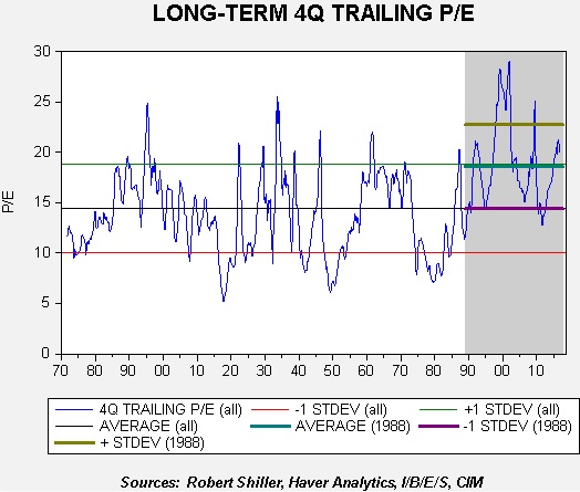
Our conclusions from Mallaby’s work tend to confirm prior comments we have made about S&P 500 P/Es. This chart shows the trailing P/E for the S&P 500; for the current quarter, we use a mix of three quarters (Q1, Q2, Q3) and consensus forecasts for Q4. The area in gray, which encompasses the period from 1988 to the present, has seen an upward shift in the P/E. Essentially, the lows recorded in this period are closer to the average observed over the entire time frame. Investors appear to have shifted their risk tolerance and are willing to “pay up” for earnings. Part of the reason why this shift occurred could be contained in the above analysis of monetary policy. The combination of expectations of central bank “rescues” from market turbulence and policy accommodation stemming from inflation targeting in a globalized economic environment may have given investors more “courage” about accepting a higher earnings multiple than seen in the past. Thus, the current P/E, though historically elevated, may not be all that risky…as long as the monetary policy environment doesn’t change.
[1] Mallaby, S. (2016). The Man Who Knew: The Life and Times of Alan Greenspan. New York, NY: Penguin Press.
[2] Ibid. Greenspan disputed Mallaby’s claim that the former was responsible for letting Burns know how he could get the rumor squelched, pp. 141-144. Mallaby stands by his position.
The November elections have had a significant impact on the financial markets. It is important to watch how policies from the new administration unfold.
We don’t expect new policies to rapidly accelerate economic growth. However, we do expect growth to improve modestly in 2017.
Our equity allocations are entirely domestic. We shift allocations toward large caps for conservative investors, while focusing more on small and mid-caps for aggressive investors.
We shorten the average maturity of bond allocations, recognizing tighter Fed policy and the potential for higher inflation.
Our growth/value style bias shifts in favor of value at 30/70.
ECONOMIC VIEWPOINTS
Since November, the outcome of the elections has dominated the market narrative. Equity markets rallied sharply, while bonds declined, reflecting a shift in expectations for higher economic and earnings growth, along with rising inflation and tighter Fed policy. Seemingly, the new expectations reflect a lot of optimism for the new president. The thing is, the elephant in the room isn’t really an elephant…at least not a traditional one. Trump made his way into the White House campaigning on positions contrary to several long-standing Republican policies. So, as we begin life under this new administration, we’ll be keeping a close eye on its policies. We’ll be watching to see if Trump tacks toward Republican supply-side views, or if he instead hews to populist priorities.
A supply-side approach would focus on making capital more available and more easily invested. Policies would include lower taxes and less regulation, with the belief that rising capital efficiency would stimulate the economy. Theoretically, companies would hire more workers and increase long-term investments. Some of Trump’s cabinet selections indicate this may be the direction he is headed toward.
On the other hand, Trump’s vocal opposition to the current state of global trade hearkens to a populist view, one contrary to decades of establishment policy. Here the expectation is for “level” global trade agreements to bring jobs back to the United States and increase wages, which would stimulate economic growth. Early jawboning indicates this may be the new policy direction.
Of course, it’s possible we see a combination of supply-side and populist policies. Unfortunately, we don’t expect either strategy to create significant job or wage growth. Technology and innovation appear to be at the root of limited labor opportunities, and both will probably play a role in disappointing some optimists. But even as we don’t expect a big uplift in growth, we do believe there’s room for some improvement in 2017. The economy has maintained a fairly steady, albeit below-average, growth rate, even as the Fed has moved through two rate increases. We believe this trend should continue with modest acceleration, unless the Fed becomes too aggressive.
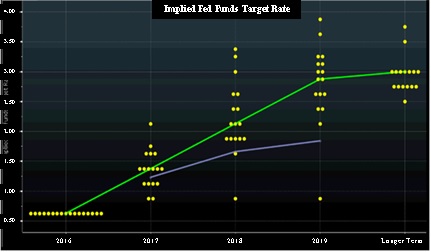
What do we expect from the Fed? Right now, Fed guidance indicates three rate hikes in 2017. Up until recently, the financial markets have been at odds with the Fed’s guidance, having expected a more moderate pace of tightening. For the most part, markets have been correct. But as we look forward, market expectations are now quite closely aligned with the Fed’s guidance. In this chart, the green line represents the median forecast for short-term rates by the Fed’s voting policy members for the next few years, while the blue line illustrates the market’s expectations. We can see the market has generally accepted the Fed’s guidance.
(Source: Bloomberg, CIM)
Will three rate hikes be too much for the economy in 2017? At this point, we don’t think so. However, even the Fed has communicated the importance of evaluating developing economic conditions as it directs monetary policy. We are optimistic the Fed can make the appropriate adjustments, even as we’re aware of the Fed’s proclivity to overtighten. Given the importance of the Fed’s policy decisions, the real elephant in the room may actually turn out to be the Fed.
STOCK MARKET OUTLOOK
Equities performed well in 2016, although most of the returns were earned after the November elections. The surge reflects widespread optimism for higher economic growth and rising corporate earnings. Although we see a pathway for both, we expect equity investors are likely to encounter periods of disappointment along the way. Valuations have risen ahead of actual results, meaning delays and shortfalls could increase downside risk.
Still, we expect a generally good environment for stocks. Small and mid-cap stocks performed particularly well in 2016, and all of the portfolios benefited from their inclusion. We continue to hold a favorable view toward small and mid-sized companies, which may benefit as Washington policies become more inwardly focused on the U.S. economy. However, with the recent strong performance of small and mid-caps, we are shifting some equity allocations toward large caps for conservative and income-oriented investors, and toward mid-caps in our more aggressive portfolios. Large caps tend to have lower relative volatility and we expect this asset class to also perform reasonably well.
Within large caps we favor the energy, financial, industrial and utility sectors, while we are underweight technology and telecom. Sector preferences incorporate our views toward valuations, industry fundamentals and potential changes in regulations. Our growth/value style bias shifts in favor of value at 30/70.
We continue to avoid foreign developed equities. Their valuations may be attractive, and many foreign economies should benefit from a stronger U.S. dollar; however, the strong dollar may also diminish returns on foreign investments for U.S. investors. Risk in emerging markets could also increase. For these reasons, we eliminate our emerging allocations this quarter and have no foreign equity allocations in the portfolios.
BOND MARKET OUTLOOK
Optimism in the equity markets following the elections was mirrored with pessimism in the debt markets. Expectations for higher economic growth benefited equities but also created expectations for tighter monetary policy, which helped move bonds lower. Adding to negative sentiment has been the prospect for rising longer term inflation, which could emerge if global trade declines.
For quite some time, we have included long maturity bonds in portfolios. This allocation not only contributed to income and returns, but it also provided significant diversification benefits. But as we look forward, we may be at the point where a multi-decade decline in rates may be turning around. If we are in a reversal, we don’t expect a rapid increase. Still, we believe it’s prudent to pare back some of the long-term bond allocation this quarter. We continue to favor corporate bonds, including both investment and speculative grades, as we expect relatively low default rates.
OTHER MARKETS
Even with an increase in longer term rates, we believe real estate can continue to perform well. Financing costs remain relatively low, while occupancy and rental rates are constructive. In addition, real estate rental rates often scale with inflation, providing a mechanism to help maintain income should inflation arise. With the modest pullback in the second half of 2016, we believe real estate is attractive, particularly where income is an objective.
Commodity prices could rise with faster U.S. growth, and this asset class may be helpful if we experience rising inflation. However at this point in the cycle, we believe other asset classes offer a more attractive return/risk profile. This quarter we exit the gold allocation, which was useful in addressing global central bank policies; however, our expectation for a strengthening U.S. dollar now makes gold relatively less attractive.
The Market
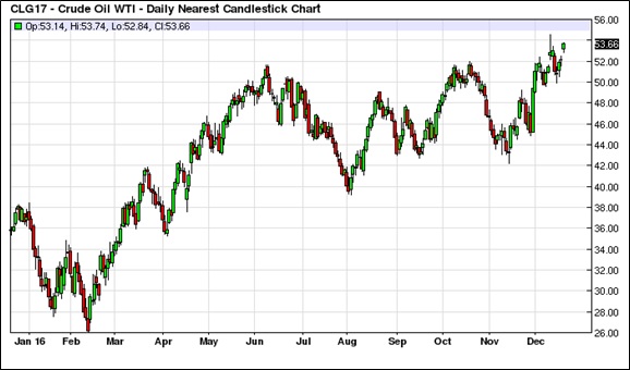
Oil prices have broken above their $44 to $52 per barrel trading range in the wake of the recent OPEC output agreement.
(Source: Barchart.com)
OPEC
In a reversal of recent policy, Saudi Arabia spearheaded an agreement to cut oil production. OPEC has agreed to cut production by about 1.3 mbpd and select non-OPEC producers have chipped in additional reductions of 0.53 mbpd as well. The total OPEC output quota is 32.7 mbpd.
The table below shows the projected cuts relative to what OPEC said it was producing (the reference column) and what Bloomberg estimated for October’s actual production. We have calculated the differences relative to quota from the two production estimates. The areas in yellow represent nations that were not awarded a quota. Indonesia is no longer an oil exporter, while Nigeria and Libya were not given a quota due to persistent production interruptions.
Due to the upcoming holidays, the next edition of this report will be published on January 6, 2017.
The Fed gave us a modest hawkish surprise last week, calling for three rate hikes in 2017 rather than two. The news has boosted Treasury yields and lifted the dollar. Equities mostly absorbed the news without incident.
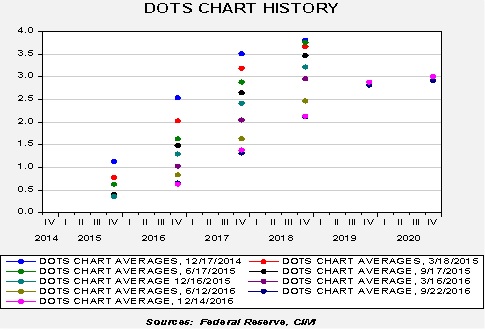
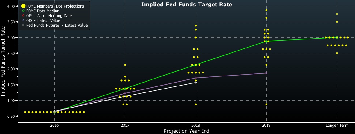
Here is a chart of the FOMC’s average dots over the past two years.
The fuchsia dots represent the most recent meeting. The dots have stopped their steady progression toward lower levels. For better or worse, the path of policy expectations from the dots suggests that the FOMC is becoming comfortable with this path of hikes.
Here is the dots plot from September.
(Source: Bloomberg)
Note the purple line, which is the LIBOR-OIS curve from the meeting day. It has jumped from where it was on the meeting date in September, shown by the red line. For the past few years, the FOMC dots have tended to decline toward the market. The rise in the LIBOR-OIS curve suggests that process is reversing.
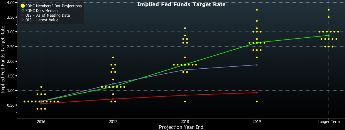
This is the new dots plot, released at the December meeting.
(Source: Bloomberg)
For 2017, the median forecast is currently 1.375%, up from 1.125% in September. For 2018, the median is up to 2.125% from 1.875%. Two participants see no change next year but one of those is probably St. Louis FRB President Bullard, who has decided not to participate in the dots procedure. Although market expectations continue to lag, we did see the LIBOR-OIS rate rise to 1.25% from 0.875% in September.
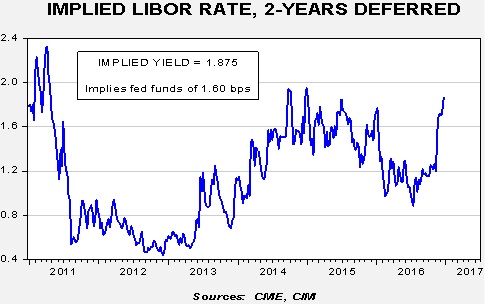
This can be seen in the deferred Eurodollar futures.
The jump in yields since Trump’s election has been striking. We are approaching the highest level of implied rates since the “taper tantrum.” This rise triggered the onset of the dollar rally in mid-2014 and we note that the dollar has been rising since the election.
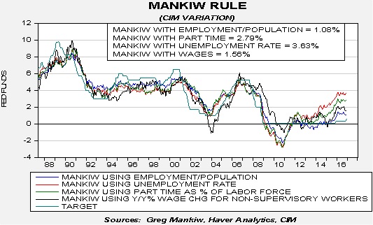
To get some sense of where policy is in relation to the neutral rate, we use the Mankiw rule model, incorporating the recent rate changes by the FOMC. This model attempts to determine the neutral rate for fed funds, which is a rate that is neither accommodative nor stimulative. Mankiw’s model is a variation of the Taylor Rule. The latter measures the neutral rate using core CPI and the difference between GDP and potential GDP, which is an estimate of slack in the economy. Potential GDP cannot be directly observed, only estimated. To overcome this problem, Mankiw used the unemployment rate as a proxy for economic slack. We have created four versions of the rule, one that follows the original construction by using the unemployment rate as a measure of slack, a second that uses the employment/population ratio, a third using involuntary part-time workers as a percentage of the total labor force and a fourth using yearly wage growth for non-supervisory workers.
Using the unemployment rate, the neutral rate is now 3.63%. Using the employment/population ratio, the neutral rate is 1.08%. Using involuntary part-time employment, the neutral rate is 2.79%. And finally, the wage growth model puts the neutral rate at 1.56%.
It is still uncertain which of these variants best reflects slack (or lack thereof) in the economy. Although we tend to think that wage growth or the employment/population ratio is the best measure of slack, the key is which one policymakers view as the most consistent with measuring slack. At this point, we don’t know, although we think the hawks are probably relying on the unemployment rate variant while the chair and most of the doves probably believe the involuntary part-time employment variant is the best measure. The involuntary part-time employment variant is most consistent with six rate hikes over the next 24 months. That path would bring the policy rate near neutral; however, if they are wrong and, for example, the employment/population ratio is actually correct, then policy will be overly restrictive (assuming that ratio doesn’t improve dramatically). Thus, the FOMC is moving rates higher in a slow fashion to allow them time to adjust if it turns out there is more slack (reflected by the lower neutral rate variants) than some data would suggest. Of course, by going slow, assuming the higher neutral rate variants are correct, the Fed could keep policy overly accommodative longer than it should. However, as long as the economy remains globalized and deregulated enough to allow for the nearly unfettered introduction of new technology, being late isn’t all that risky. That assumption would change if the incoming President Trump puts up trade barriers. Thus, the path of monetary policy could be a risk factor in the upcoming year.
The economy will avoid a recession in 2017. GDP growth is expected to average 2.8% with core PCE inflation approaching the Federal Reserve’s target of 2.0%.
Fixed income markets will be challenging:
We expect three rate hikes of 25 bps each by the FOMC;
Due to rising inflation expectations, 10-year yields will reach 3%;
A swing toward equality and higher inflation would be expected to narrow credit spreads.
Equity markets should be strong until Q4:
Basis the S&P 500, our base case is for a 9.2% rise in earnings to $119.45;
Our base P/E model is projecting a fair value of 18.4x;
Our forecast for the S&P 500 is 2400 to be achieved sometime in 2017, most likely by Q3;
Earnings should exceed our base forecast because:
We will see a narrowing of the S&P/Thomson Reuters operating earnings spread;
Corporate tax reform should increase earnings.
Multiples should also expand due to:
Improved investor sentiment over Trump’s victory, although this could wane by Q4;
High levels of “sideline” cash.
We continue to favor domestic over foreign stocks;
We have a bias toward value;
We are neutral on capitalization.
Commodity prices will tend to struggle due to dollar strength. Oil prices will average around $55 per barrel due to OPEC’s actions to reduce supply.
The dollar will remain strong. We would expect the EUR/USD rate to approach $1.00.
Note: The structure of this report will be somewhat different from our previous forecasts in that we will present a framework for the economy and markets signaled by the election of Donald Trump. We will first offer a basic outline of what Trump represents and use this framework in our forecasts for next year. There are always risks and unknowns about any new president, but the potential for error is elevated as we believe this election clearly signals a change in direction for the economy and the country. Our 2017 Outlook will be affected by these changes, requiring us to discuss at least our initial estimates of the impact of President-elect Trump.
Equity markets are expensive by numerous measures and have become even more extended in the wake of the “Trump Rally.” As noted in our weekly P/E update (found in the last section of the Daily Comment), our four-quarter measure of the P/E is elevated. Another well-known derivation of the “Buffet Indicator” has also reached lofty levels.
This ratio divides the market value of equities outstanding from the Federal Reserve’s Financial Accounts of the U.S. by GDP. Although the ratio is off its recent highs, it is still at the upper end of its historical range.
At the same time, the optimism isn’t unfounded. Proposals for corporate tax reform could bring repatriation of the more than $2.0 trillion of corporate cash parked overseas. Tax cuts would boost after-tax earnings. The “E” part of the P/E could rise, making the market less expensive. Another factor to note is that investor cash levels remain elevated.
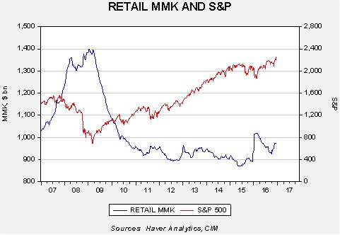
This chart shows the level of retail money market funds relative to the S&P 500. Since 2011, equities have tended to trend higher when money market fund levels exceed $920 bn. Once money market holdings fall below that level, equities have tended to stall. It appears that investors were building cash in front of the election but, so far, retail investors are not aggressively entering the equity markets. The weekly mutual fund flows suggest that investors are selling out of bonds which probably accounts for the recent rise in money market funds; to date, there isn’t any evidence in the same data that equity mutual fund buying is increasing. This data would suggest that there is ample fuel for further gains in equities.
So, if equities are rich but could work higher, how high is high?
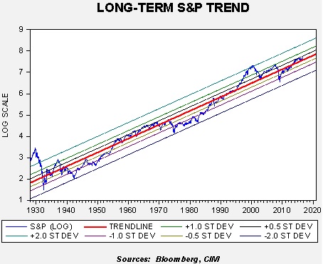
On this chart, we log-transform the weekly close of the S&P 500 starting in 1928. The red line is the long-term trend. We have regressed the trend line against the weekly close and have calculated the standard deviation at the ½ level, one deviation and two deviations from trend. Only twice in the past 88 years has the index exceeded two standard deviations to the upside and it has only touched that level on the downside three times. We are currently below ½ deviation on the upside, suggesting that, on a long-term trend basis, equities are not all that extended.
If we reach +½ standard deviation by mid-2017, the S&P 500 would reach 2480.70; the year-end reading would be 2562.22 by the same measure. By comparison, reading the +one standard deviation line would put the index at 2995.80 by June 2017, and 3094.24 by year’s end. We are not anticipating a rise to +one standard deviation next year but a rise to the +½ level isn’t out of the question.
We still don’t know what the specific policies will be of the incoming Trump administration. Tax policy is complicated and there is always the potential for mistakes. The current euphoria surrounding other policies will probably fade over time. And, although the above analysis suggests that equity markets are sporting high valuations, cash levels are high and current equity levels, while above trend, haven’t reached levels of concern. Thus, for the time being, the path of least resistance for equities is probably higher.
We use cookies to ensure that we give you the best experience on our website. If you continue to use this site we will assume that you are happy with it.