by Asset Allocation Committee

Does the Federal Reserve adjust policy for asset prices?  This is perhaps one of the most controversial topics in U.S. monetary policy.  Alan Greenspan faced this issue in the early 1990s.  Both Volcker and Greenspan wanted to focus monetary policy on containing inflation.  But, Larry Lindsey, a Fed governor at the time, noted that if outside forces, such as technology and trade, were keeping inflation down then the Fed could engage in easy monetary policy without the risk of rising price levels.  He warned this could cause asset bubbles.[1]  Greenspan, an adept corporate infighter, prevented Lindsey’s position from gathering any momentum.  But, as the “irrational exuberance” speech showed on December 20, 1996, he became concerned about overheating financial markets.[2]   However, the reaction to the speech led the powerful Greenspan to realize there wasn’t much upside in conducting monetary policy to quell asset bubbles.  Instead, policy evolved to address the aftermath of bubbles.

Still, the idea of low interest rates triggering asset inflation never really went away.  The Great Financial Crisis proved that the costs of cleaning up after a bubble could be considerable.  It was one thing to have a bubble in technology stocks; in general, technology becomes obsolete so quickly that excess capacity in that sector doesn’t have a lasting effect.  On the other hand, a bubble in housing can depress economic activity for years.  Jeremy Stein, a Fed governor from 2012 to 2014, raised concerns about financial excesses.[3]

In the current configuration of the FOMC, shown below, we rate them according to their policy bias (on a 1 to 5 scale, with 1 being the most hawkish and 5 most dovish) and by theoretical inclination.  The latter reflects traditional hawks, characterized by a restrictive view of the Phillips Curve, traditional doves, who have an expansive view of the Phillips Curve, moderates, who make policy based on a variety of factors but tend to be “data-dependent” (in practice, atheoritical and not tied to the Phillips Curve) and financial asset-sensitive.  The table below shows the breakdown.  The number shows policy bias based on our analysis of comments and voting patterns.  The colors show what we view as their theoretical background.  Among the voters this year, the average is nearly 3, suggesting a moderate voting bloc.  This year, there is only one dove and one hawk, five moderates and three financial market-sensitive voters.  The doves tend to raise rates reluctantly; hawks tend to cut rates with the same distaste.  Moderates are mostly a diverse group from a theoretical perspective.  For our purposes, the important difference of this group compared to the traditional hawks and doves is skepticism about the Phillips Curve.  These voters tend to watch trends in the overall economy and make policy decisions.  Interestingly enough, three of the governors appointed by President Trump have been moderates and he also promoted Jerome Powell to chair of the FOMC.  For a president who seems to prefer doves, he has been steered into appointing moderates.  Finally, there are three members who, in the comments, seem much attuned to the behavior of financial markets.  Governor Brainard has voted as a dove but has expressed concern about market overheating and has used that position to support recent rate hikes.

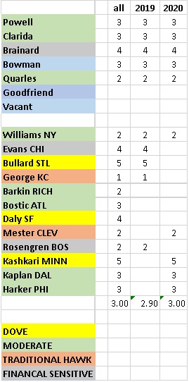
This year, we have three voters we dub as “financial-sensitive.”  Thus, financial market behavior may be important to the path of policy this year.

However, as Greenspan noted, it’s hard in real time to determine whether an asset market is in a bubble.  And, it can be equally difficult to determine whether the cost of raising rates to prevent the bubble is less expensive than addressing the aftermath.  The key problem with asset bubbles is that they leads to malinvestment.  In a long-lasting asset, that can mean years of technical inefficiency because capacity can’t be fully utilized.  Thus, a housing bubble can lead to too much real estate that can take years to absorb; cutting interest rates can help slow the inevitable decline in prices but may actually expend the period necessary to balance the market.  On the other hand, a bubble in wheat lasts one growing season and policymakers shouldn’t bother to address the problem.

In addition, it would be politically explosive for policymakers to raise rates solely because equity or home prices have risen “excessively.”  The backlash would threaten central bank independence.  Thus, if the Fed is worried about an asset bubble, it would need some measure other than valuation to raise rates.

One possibility we have examined recently is volatility.  Does the FOMC adjust rates based on the equity market VIX?  There appears to be some evidence that policymakers may be sensitive to market volatility.

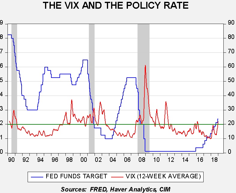
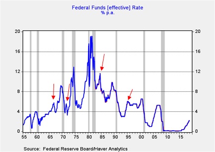
This chart shows the weekly fed funds target with the 12-week average of the CBOE VIX index.  We have placed a bold line at 20 for the VIX.  Since the late 1990s, we note that the FOMC was inclined to keep lowering rates with a VIX above 20; a reading under 20 would tend to support policy tightening.  So, in 2002, Chair Greenspan kept cutting rates even though the economy was in clear recovery.  It may have been due to perceptions that investor sentiment was overly negative.  The 2004-06 tightening cycle occurred with a VIX persistently below 20.  In fact, rate cuts seemed to occur as the VIX rose.  We also note that the 2016 pause occurred after the VIX rose back above 20, and tapering was announced in 2016 after a prolonged period of a low VIX.  The current pause coincides with the recent lift in volatility.

We also examined adding the VIX to the Mankiw Rule model variations.  What we found is that the index is statistically significant in three of the variations and the correct sign in two.  However, in the variations it did correctly affect, it didn’t necessarily improve the forecasting accuracy by more than 10 bps.  This performance suggests that the VIX may have an impact on policy but the Phillips Curve variables, labor market data and inflation, are still more important.  However, the hard part to divine is the impact of the VIX on the moderate voters.  Even if all of the market-sensitive members pay attention to the VIX, the moderates may only pay attention at extremes.

Therefore, in conclusion, we can probably say the following—when the VIX is below 20, the Fed is probably more likely to consider tightening policy.  A reading above 20 may lead to a pause or could encourage further easing.  However, the relationship isn’t precise, which suggests the traditional hawks and doves don’t pay much attention to market volatility.  The VIX may be the way that market-sensitive FOMC members can incorporate financial markets into their policy decisions without overtly targeting valuations or returns.

View the PDF

---

[1] Mallaby, Sebastian. (2016). The Man Who Knew: The Life and Times of Alan Greenspan. New York, NY: Penguin Books. (pp. 435-36.)

[2] Ibid, pp. 504-506.

[3] https://fraser.stlouisfed.org/title/1163/item/2372 and https://fraser.stlouisfed.org/title/1163/item/476707

by Asset Allocation Committee

Quantitative easing (QE) was an element of unconventional monetary policy that emerged from the Great Financial Crisis.  When the Federal Reserve lowered the fed funds target to zero (known as the “zero interest rate policy,” or ZIRP), policymakers decided that taking the policy rate below zero would not further stimulate the economy.  Once interest rates fall below zero, idle cash generates a return and there was fear that negative interest rates would cause cash hoarding, which was exactly what the Fed wanted to avoid.  However, policymakers also feared that signaling they lacked additional tools to support the economy could trigger a panic in financial markets.  Thus, they created an additional tool, QE, which bought Treasuries and mortgages from the financial system and pushed additional cash into the economy.

The policy was controversial.  Some feared it would trigger inflation as the high levels of cash would “inevitably” cause rising prices.  Others argued that the process would distort financial markets.  But, in the end, the effects of QE were difficult to parse.  For example, one of the Fed’s arguments for QE was that it would lower long-term interest rates.  In fact, at times, it seemed to have precisely the opposite effect.

This chart shows the 10-year T-note yield.  The gray bars show periods of QE.  In all three events, yields rose at the onset of the balance sheet expansion.  Yields eventually fell during QE2, although that decline was probably more due to turmoil in Europe.  Why did yields rise when the Fed was reducing the supply of bonds?  Most likely, investors worried that QE would be successful in bringing about inflation and thus demand was adversely affected.  Anticipation of the end of QE always led to a drop in yields.

What about all that money that was injected into the system?  Much of it remained on bank balance sheets in the form of excess reserves.

Using the equation of exchange (money supply x velocity = price x quantity), the increase in the money supply mostly led to a sharp drop in velocity, instead of boosting prices or quantity.

So, if QE mostly sat idle on bank balance sheets then the withdrawal of QE should not have had much of a real impact on the economy.  And, that is likely true.  However, this isn’t to say that QE had no effect.  As we have noted in the past, there has been a close correlation between the S&P and the Fed’s balance sheet.

The chart on the left shows the original balance sheet model; note that after Trump’s election in 2016 the S&P rose much more than the model would have projected.  To account for this move, we built a variable that adjusted for expectations surrounding corporate tax cuts.  The additional variable improved the model dramatically; however, assuming no further reductions in corporate tax rates, the market is once again tracking the balance sheet.

Essentially, it appears that the impact of QE was mostly psychological; it signaled to investors that the Fed was supportive.  Interestingly enough, the withdrawal appears to be adversely affecting investor sentiment.  It is hard to determine how much, simply because there are other factors, such as trade conflicts and FOMC criticism, which are also affecting sentiment.  However, this data suggests that a pause in the balance sheet reduction would likely improve investor sentiment.

View the PDF

by Asset Allocation Committee

(N.B.  This is the last Asset Allocation Weekly for 2018.  Have a Merry Christmas and Happy New Year.  The next report will be published January 4, 2019.)

The U.S. economy is performing in line with the rest of the world.

This chart shows the yearly change in U.S. and world ex-U.S. GDP.  The lower line on the chart shows the difference.  On average, U.S. growth is usually 0.61% lower than world growth and the world exceeds U.S. growth 70% of the time (with data since 1981).  This situation isn’t a huge surprise; the U.S. is the world’s largest economy and smaller economies can grow faster more easily.  The lower line shows that U.S. growth has been gaining on world growth for the past two years.

The net number does coincide with dollar cycles.

When the growth differential is below average (implying stronger world growth relative to the U.S.), the JPM dollar index averages 107.21.  When growth exceeds average, the index averages 113.14.  We are projecting slower growth in the U.S. next year, around 2.7%, which is essentially average growth.  If world growth also holds near average, around 3.3%, it would be reasonable to expect the dollar to weaken from current levels.  The U.S. growth surge in 2015 led to a strengthening dollar and this year’s rally was partly due to the lift in U.S. growth due to fiscal stimulus.  As that wanes, relative growth should favor the world, which will support a softer greenback.  In general, a weaker dollar will tend to support commodities and foreign equities, especially emerging markets.   We expect those assets to perform better in 2019.

View the PDF

by Asset Allocation Committee

Equity markets have come under pressure this autumn.  The weakness has gained momentum in recent weeks.

This chart shows the yearly change in the S&P 500 Index on a monthly average basis.  We have added recession shading; in general, recessions tend to trigger bear market declines of 20% or more.  In fact, every decline of this magnitude has been associated with a downturn in the business cycle since the 1987 Crash.

There have been two sources of recent weakness.  The first is fear that the Federal Reserve will make a policy error and trigger a recession.  These fears are not unfounded.  Since the mid-1950s there have been 13 tightening cycles; only four have resulted in a “soft landing,” a cycle that didn’t trigger a recession.

This chart shows the path of fed funds since 1955, shortly after the central bank became independent of the Treasury.  We have placed arrows where tightening cycles didn’t bring a downturn.  As the chart shows, it’s rare for the Fed to avoid a downturn.  It should be noted that the second arrow coincided with the Nixon price and wage freeze; Chair Burns likely lowered fed funds in response to the price freeze.  Thus, we can make the case that there were only three soft landings that were independently engineered by the Fed.

The second concern is over trade policy.  The administration’s trade policy threatens to disrupt supply chains tied to China which could lead to shortage and higher prices for various goods.  The impact of this outcome is very difficult to estimate; we haven’t had an aggressive policy of trade impediments since the 1920s.  At the same time, it should be noted that trade frictions are partly a negotiating stance.  These issues can be adjusted given the economic and political climate.  Since next year is the last full year before elections, we would not be surprised to see some moderation of the Trump administration’s stance on trade policy.

If the FOMC does manage to bring a fifth soft landing and we see some moderation of trade policy, the equity market may be poised for a recovery.  Since the late 1990s, the ISM manufacturing index has been a reasonably good indicator of the S&P 500.

This chart compares the yearly change in the S&P 500 Index monthly average against the ISM Manufacturing Index.  The equity index, relative to the perspective of U.S. manufacturing purchasing managers, should be up 22.1% from last year; that would put the index at 3259.27.  Not only that, but the current reading is at levels consistent with recession.  This analysis suggests that if recession is avoided in 2019 then the equity market could be poised for a strong recovery.  Essentially, this model is saying there is a disconnect between the economy and equities.  These disconnects occur occasionally but the current one stands out as extreme.  Therefore, there may be more risk to reducing equity exposure in the current turmoil.

View the PDF

by Asset Allocation Committee

The election of Donald Trump has been characterized as part of a populist uprising.  In the president’s inaugural address, he talked about the “forgotten” that would have a voice in his administration.  At the same time, we work under John Mitchell’s dictum of “watch what we do, not what we say.”[1]

In a recent Bloomberg podcast, Edward Alden, a journalist and fellow at the Council on Foreign Relations, was asked if the Trump administration favored business or labor.  He replied that they are trying to help both.[2]  We think Alden is correct in his assessment which is one of the reasons why analyzing the direction of policy with this administration is so difficult.  It appears that one of the goals of the president’s trade policy is to bring production back to the United States which would benefit labor.  At the same time, tax policy has generally favored capital.  But, the most underestimated benefit to capital may be deregulation.

George Washington University measures the pages of the Federal Register, which is the official journal of the federal government.  It publishes agency rules, proposed rules and public notices.  So, the number of pages in the register says something about the number of regulations.  The idea is that the more pages added to the register signals an increase in regulation.

The decline seen in the first full year of the Trump administration is remarkable.

The drop from 2016 to 2017 was 35.4%, which exceeds the 21.2% decline in 1981, Ronald Reagan’s first full year in office.  The only year that was larger was 1947, which saw a 39.6% slide.  That drop was likely due to postwar changes.

Another measure is called the “significant rule changes,”[3] a policy measure created during President Clinton’s first term.  The decline in 2017 was unprecedented.

Only 55 new rules were added in 2017.  That is clearly the fewest on record by multiples.

The drop in regulatory activity is partly why small business sentiment has been so strong.

The jump in small business sentiment mostly tracks the drop in regulation.  A persistent complaint from small business leaders during the Obama administration was the regulatory burden.  Not only did President Trump promise to reduce regulation, he actually accomplished it.

Tax changes and deregulation have been supportive factors for equities since the November 2016 presidential election.  However, as Edward Alden noted, the Trump administration has tried to placate both capital and labor.  Recent market action, with equities selling off despite a civil meeting between Presidents Trump and Xi and the yield curve flirting with inversion,[4] suggests that the financial markets are pressing President Trump to choose.  Will it be capital or labor that wins out in the end?  If capital is going to win, a lasting trade ceasefire needs to be declared.  If President Trump sticks with tariffs, and there are ample indications that he intends to for now, then the financial markets appear to be preparing for recession.  A recession in 2019 will jeopardize the president’s chances at reelection in 2020.  Our expectation is that, at some point, President Trump will “blink” and tone down the trade rhetoric.  But, that is an open question for now.

View the PDF

---

[1] http://www.arlingtoncemetery.net/mitchell.htm

[2] https://www.bloomberg.com/news/audio/2018-11-27/surveillance-china-general-motors-with-cfr-s-alden-podcast Alden’s segment begins at 16:00 minutes and the response in question is at 18:40.

[3] https://www.reginfo.gov/public/jsp/Utilities/EO_12866.pdf and summarized https://www.epa.gov/laws-regulations/summary-executive-order-12866-regulatory-planning-and-review

[4] For an analysis of the impact of inversion, see our Asset Allocation Weekly (6/29/18).