by Asset Allocation Committee

As various permutations of the yield curve invert, projections of recession are increasing.  One of our favorites, the 10-year T-note/fed funds yield curve, has been inverted for three months.

This chart shows the history of this yield curve; since 1960, every recession was preceded by an inversion of this indicator.  However, that isn’t to say that every inversion led to a recession. There were two false positives in the series, one in 1965 and another in 1998.  The former we consider a true false positive as the inversion lasted several months but a recession didn’t follow.  The latter event only lasted one month and was tied to the financial turmoil of the Asian Economic Crisis, the collapse of Long-Term Capital Management and the Russian debt default.  The fact that the inversion was short-lived weakens the case that it was a true inversion.

If this signal of recession holds, when does it arrive?  Here is a look at the timing:

On average, recessions occur 15 months after inversion; that would put the onset around next September.  The range is eight months to 18 months.  Using that range, the recession could begin as early as February 2020 or as late as February 2021.  Although this history offers some insight into timing, the reality is that the number of events is rather limited.  Thus, investors should treat the data as a guide.  The economic data remains mixed, but the preponderance of the evidence suggests that the U.S. economy is weakening but not in recession.

As we have noted before, recessions tend to have two causal factors, policy error and geopolitical events.  The 1973-75 and 1990-91 recessions are considered to be partly due to geopolitical factors; the former was affected by the Arab Oil Embargo and the latter by the Persian Gulf War.  However, both also had yield curve inversions.  It is quite possible that the geopolitical events caused the recessions to occur faster than they might have otherwise in the absence of these events.

We are watching the trade conflict with great interest because it might affect the timing of a downturn.  If the trade conflict worsens, lifting import prices and forcing the Fed to slow its path of lowering rates, the recession might occur sooner than it otherwise would.  A recession would certainly affect the 2020 elections; no incumbent has survived a recession since Calvin Coolidge.  We will likely begin to prepare for a downturn next year.  If the trade conflict worsens, the timing may be accelerated.

View the PDF

by Asset Allocation Committee

Recession worries have increased due to falling long-duration interest rates and the short-lived inversion of the two-year/10-year T-note spread.  Although this spread is important, it is merely one in a whole series of permutations of the yield curve.  Our preferred measure is the 10-year/fed funds spread because it measures the long end of the yield curve to the policy rate and thus should provide a clearer picture of whether or not the central bank policy is too tight.  It is also the same spread the Conference Board uses in its leading economic indicators.

This chart shows the aforementioned spread.  Since the 1970 recession, the spread has inverted before every recession.  It did have two false positives, one in 1966 and another in 1998.  The recent inversion could be a false positive as well, but it makes sense that investors should be concerned about a recession.  This is because equities often decline during recessions; in some cases, the drop is significant.

This chart shows the weekly Friday close for the S&P 500 on a log scale.  We have regressed a time trend through the data.  In nearly all recessions, some weakness in equities is observed, although often the decline in stocks predates the recession to some degree.

This chart shows the performance of the S&P 500 around inversions.  We took every inversion from 1966 forward, indexing the S&P to 100 at the month of inversion.

We added symbols to the 1966 and 1998 inversions as both were false positives for recession.  In the former case, equities fell in the first 10 months of inversion but rallied.  In 1998, there was a brief drop followed by a strong rally in stocks.  Generally speaking, false positives are buying opportunities.  All the other events were eventually followed by recessions.  However, as the data shows, the dispersion is remarkably wide.  It’s hard to ascertain a clear message with this much noise, but, in general, a case can be made that a delayed recession after inversion tends to support equity values.  The other message is that valuations and inflation issues do matter around inversions.  The worst performing markets in the two years after an inversion was 1973, a bear market that suffered from falling margins and multiples, and 2000, which was a highly overvalued equity market.  Other than these lessons, the data tends to support the idea that panic around an inversion is probably unwise, which is what the average of all the events tends to suggest.  Each inversion has specific characteristics that affect equity market performance.  In the current environment, we would be most concerned about profit margins; if a recession occurs, we would expect margins to contract which would likely trigger a notable bear market.  So far, margins have declined but remain historically elevated.  Margins will likely be the key to equity performance in the coming quarters.

View the PDF

by Asset Allocation Committee

As the 10-year T-note yield tumbles, we are reaching a point where the market looks overvalued based on current fundamentals.

Our yield model uses fed funds and the 15-year average of the yearly change in CPI[1] along with the JPY/USD exchange rate, oil prices, the yield on 10-year German bunds and the fiscal deficit as a percentage of GDP.  The current yield on the 10-year T-note, dipping below 1.70%, puts the deviation from fair value at nearly a standard error below fair value.  Not every deviation from fair value is resolved through higher interest rates; sometimes the fair value yield declines.  The last time we saw this sort of event occur was in 2012 during the Euro crisis and the U.S. Treasury downgrade.  That proved to be an unsustainable low in yields.  We also saw a dip in early 2008; that issue was resolved by falling T-note yields due to the financial crisis.

Isolating fed funds and assuming the rest of the variables remain steady shows that the bond market has factored in a fed funds of 10 bps, or essentially a return to ZIRP.  To be fair, it is also possible that the financial markets are lowering estimates of inflation.  The 5-year/5-year TIPS calculation[2] puts the forward inflation rate at 1.80%; our long-term average calculation is around 2.08%.  Applying that inflation rate expectation into the model means the current T-bond yield has discounted a 50 bps fed funds rate.

In any case the bond market is essentially making the case that a recession is likely.  If a recession is avoided, we would expect to see a significant rise in long-duration yields.  For now, the uncertainty surrounding trade and weakening global growth will probably continue to support a long-duration position.  But, given the mercurial nature of the trade discussions, a rapid reversal is not out of the question and thus requires close monitoring. 

View the PDF

[1] This variable acts as a proxy for inflation expectations.

[2] This series is a measure of expected inflation (on average) over the five-year period that begins five years from today.

by Asset Allocation Committee

Since the end of WWII, there have generally been three factors that have caused recessions.  The first, and most important, is policy error.  Although fiscal tightening can cause recessions, major tax increases have become less common.  The usual source of policy error comes from the monetary side, where the central bank either raises rates too high or doesn’t move quickly enough to lower rates when business conditions weaken.  The second cause comes from geopolitical events.  The 1973-75 recession was triggered by the Arab Oil Embargo, a direct result of U.S. aid to Israel during the Yom Kippur War.  The 1990-91 recession was due to the Persian Gulf War.  The third cause is due to inventory mismanagement.  The third reason has become rare due to improved logistics technology.  Although inventory issues can affect sectors of the economy, it hasn’t led to a national downturn since the 1950s.

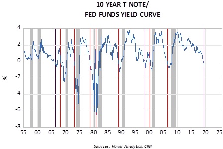
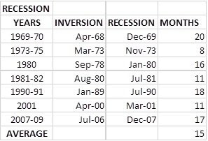
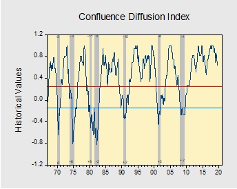
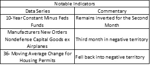
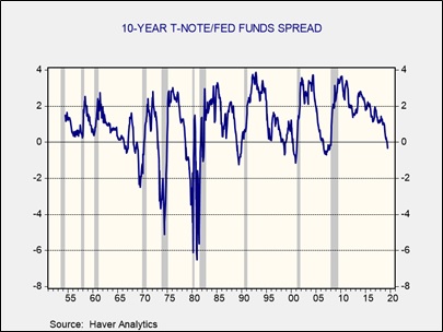
As a result, currently, there are two factors we watch most closely to predict recessions, monetary policy and geopolitical issues.  Although predicting recessions is difficult, at least with monetary policy, there are consistent indicators, such as yield curves, financial stress indexes, volatility indexes, Phillips Curve measures, etc.  Obviously, timing is difficult, even when the indicators flash warning signs, but at least there are fairly consistent indicators one can monitor.

Geopolitical indicators are far more idiosyncratic.  Global tensions are constant.  There are always geopolitical tensions so it is hard to parse the signal from the noise.  To some extent, this is always a problem with geopolitics.  It’s not that there is a lack of situations that could develop into a threat to the business cycle; it’s just that most don’t.

Perhaps a better way to think about geopolitics and theor impact comes from the book, Ubiquity: Why Catastrophes Happen.[1] In this book, Mark Buchanan makes the case that geopolitical events are much like sandpiles where grains rise steadily, making the structure increasingly unstable.  A final grain triggers a collapse and, due to the post hoc, egro propter hoc fallacy, that last “grain” becomes the “cause” of the collapse.  In reality, the structure had been losing stability for some time and the triggering event may not have led to the catastrophe under conditions of stability.

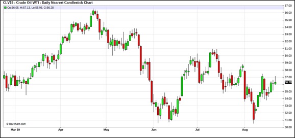
For example, the Persian Gulf War occurred mostly because Saddam Hussein miscalculated the reaction of the world to his invasion of Kuwait.  He probably would not have invaded Kuwait if the Kuwaitis had been willing to reduce production to allow Iraq to have a greater market share of world oil markets, something that Iraq felt it was owed from the Persian Gulf states due to its prosecution of the war against Iran.  In addition, if the Soviet Union hadn’t collapsed, Moscow would have probably not supported the invasion by its client state.  The trigger to the war, the reports that Kuwait was using horizontal drilling to tap Iraq’s oil fields, was the proximate cause of the war.  But, the mere act of taking the oil may not, by itself, have triggered the invasion without the other factors in play.

The current trade conflict with China has similar complicated characteristics.  The U.S. has been struggling to develop a consistent foreign policy since the end of the Cold War.  Policy toward China has mostly been to support its economic development on the idea that the richer it becomes, the more likely that it will democratize, following the path of other Asian nations.  Unlike Japan, South Korea and Taiwan, however, China was not as reliant on American security.  Those nations were directly protected by the U.S., whereas China only relied on America’s sea lane security.  In addition, China viewed its commitment to communism as something to be maintained.  The construct of the Trans-Pacific Partnership, which was designed to isolate China, showed that the U.S. was rethinking its relationship with China by 2008.

Under President Trump, the relationship with China has become increasingly contentious.  The application of tariffs and continued negotiations have caused increasing equity market turmoil.  Nevertheless, so far, the impact on the economy has been less dramatic.  However, we may be reaching the point where the trade conflict will begin to affect the economy.  The most recent decision by the Trump administration to apply 10% tariffs on $300 bn of imports, by itself, is probably not enough to trigger a downturn.  But, the culmination of earlier tariffs and the impact to technology restrictions may be creating conditions that lead to recession.

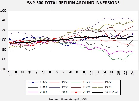
History suggests that recessions induced by geopolitical events are difficult to avoid even with stimulative economic policies.  The unknown is whether we are near a point where geopolitical risks are great enough to trigger a downturn.   At this point, we are probably not at that level but risks are escalating and the odds of a geopolitical mistake are rising.  Although it is probably too soon to position portfolios in a defensive manner, tactical planning is in order.

View the PDF

[1] Buchanan, Mark. (2000). Ubiquity: Why Catastrophes Happen. New York, NY: Three Rivers Press.