Weekly Energy Update (November 18, 2021)

Posted on November 18, 2021November 18, 2021 by Donna O'Donnell

by Bill O’Grady, Thomas Wash, and Patrick Fearon-Hernandez, CFA | PDF

(N.B. Due to the Thanksgiving Day holiday, the next report will be published on December 2.)

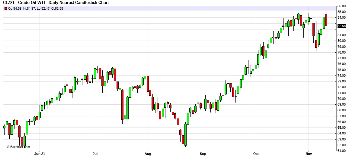
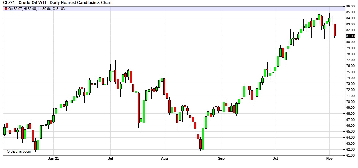
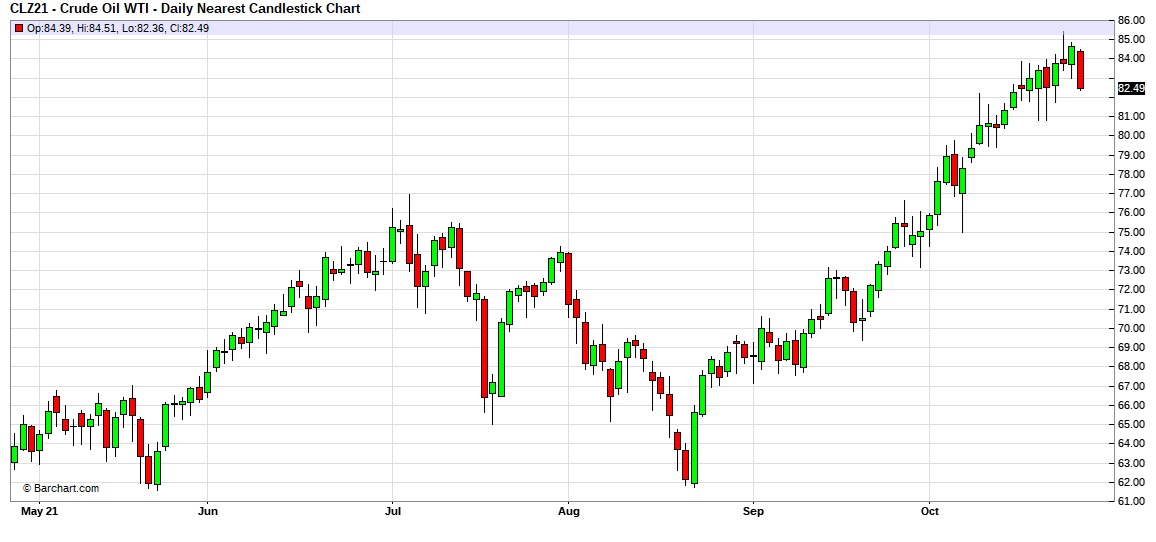
Oil prices have been struggling this week, testing support $79.50.

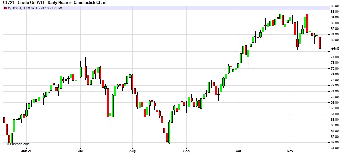(Source: Barchart.com)

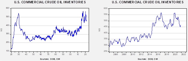
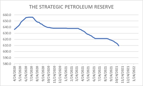
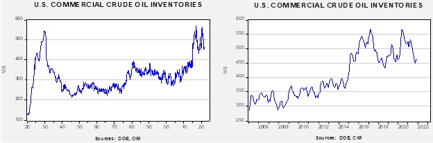
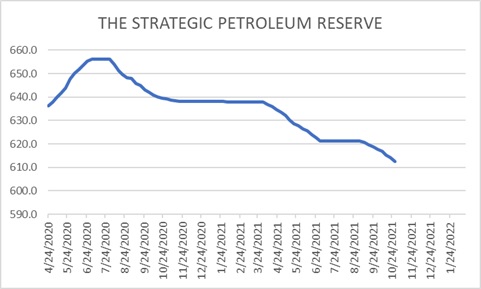
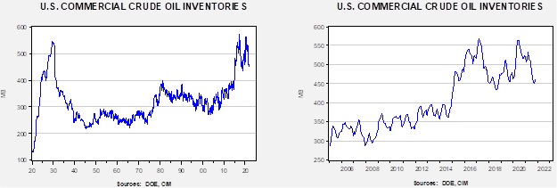
Crude oil inventories unexpectedly fell 2.1 mb compared to a 1.2 mb build forecast. The SPR declined 3.2 mb, meaning the net draw was 5.3 mb.

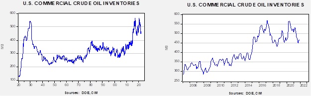
In the details, U.S. crude oil production was unchanged at 11.5 mbpd. Exports rose 0.1 mbpd, while imports fell 0.1 mbpd. Refining activity rose 0.4%. This build season usually ends in mid-November.

(Sources: DOE, CIM)

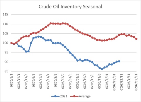
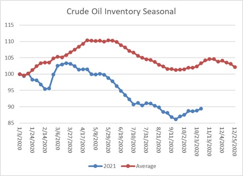
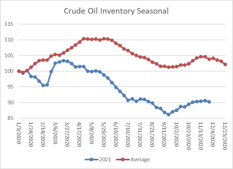
This chart shows the seasonal pattern for crude oil inventories. We are nearing the end of the autumn build season. Note that stocks are significantly below the usual seasonal trough. Our seasonal deficit is 70.0 mb.

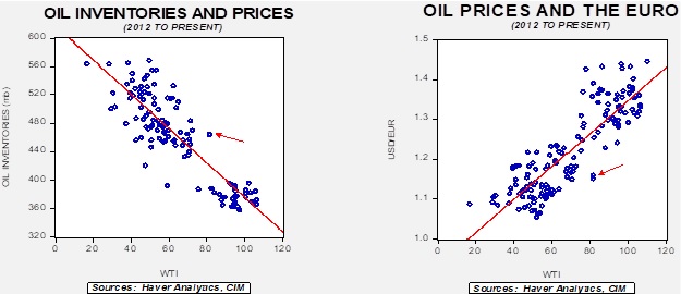
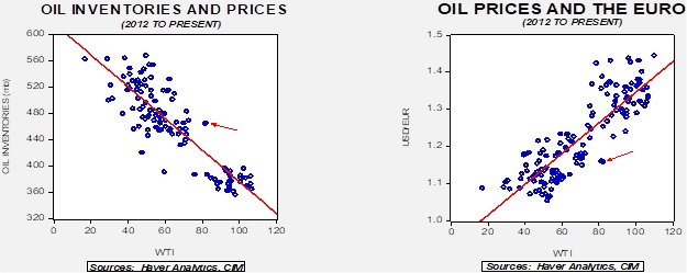
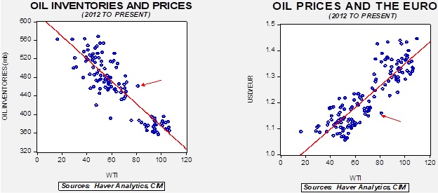
Based on our oil inventory/price model, fair value is $63.80; using the euro/price model, fair value is $56.63. The combined model, a broader analysis of the oil price, generates a fair value of $59.77. Across all models, the current price of oil is overvalued. The biggest concern has been dollar weakness, which is creating a serious divergence in the model. Although we have been bearish about the dollar because of purchasing power parity factors, we suspect foreign governments prefer dollar strength and are taking advantage of the benign neglect of U.S. dollar policy.

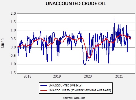
One factor we are watching is that the trend in unaccounted for crude oil is elevated. The most likely reason is that production levels are being underestimated, and, if so, the 12-week average would suggest that production is +0.5 mbpd higher than being reported.

Market news:

The Biden administration faces political pressure from high oil prices and is trying to craft a response. There has been talk of a larger SPR release, curtailing oil exports, and easing ethanol blending requirements. All these proposals carry risks. A larger SPR release could leave the nation vulnerable to a crisis in the Middle East. Although the U.S. has an ample reserve, the goal of SPRs is to reduce hoarding, so it has to be large enough to overcome that psychological hurdle. Curtailing exports to a world in shortage isn’t how a superpower behaves and would undermine the “America is back” policy of this administration. Reducing biofuel blending would anger the farm sector. So far, the administration is using the “round up the usual suspects” approach by claiming market manipulation. We have covered energy markets since 1989, and, to our knowledge, there has never been a demonstrated case of market manipulation. At the same time, numerous presidents have pressed the FTC to conduct investigations.
- It should be noted that the administration wants a methane tax designed to punish drillers, pipelines, and processors over natural gas leaks. Unfortunately, the tax will likely lift natural gas prices at a time when supply concerns have boosted price levels.
The IEA is upbeat about higher supplies in the coming months. The U.S. is holding a large offshore permit sale soon. It will be interesting to see the level of interest in projects that may not provide new supplies until early 2030. Meanwhile, Permian Basin production is set to rise next month to a new record.

Geopolitical news:

Although Iran and the U.S. continue to signal a return to JCPOA, the reality is that neither side has a singular vision on what that means. Iran wants assurances that a new administration would not exit again. It isn’t possible unless the U.S. makes a treaty, and there is no way the Senate would support a full treaty. Iran also wants the U.S. to admit fault in leaving, which isn’t likely either. Meanwhile, Iran continues to make progress in nuclear technology and won’t likely give that up in a new arrangement.
Recent elections in Iraq are leading to rising tensions among Shiite groups. Some of these groups are aligned with Iran, others are not, and the two sides are increasingly prone to conflict.
The Iranian Revolutionary Guard Corps is increasingly encroaching on the Kurdish areas of Iraq.
Iran has been a staunch ally of the Assad regime in Syria, backing the family during its civil conflict. The Arab states in the region would have preferred to see the Assad family ousted, but as it becomes increasingly evident the regime is going to survive, Arab states are making tentative overtures to Damascus. Syria has been a crossroads of the region; Syrians are used to managing relationships with states in conflict. Syria would likely support normalization with the Arab nations to assist in rebuilding, but it isn’t likely Tehran will look kindly on this development.
Turkey is systematically constraining water supplies to Syrian Kurds. The Erdogan regime views the Syrian Kurds as supporting Kurdish separatism.

Alternative energy/policy news:

COP26 ended on a disappointing note, as China and India prevented a proposal to reduce coal consumption more rapidly. Both nations rely heavily on coal for electricity production, and the recent energy shortages in China have highlighted how dependent the country is on coal. As we noted last week, these arrangements are prone to free-rider problems, so the promises made were generally compromised.
- Politically, there is a risk if the burden of adjustment to the curtailment of fossil fuels falls on lower-income households.
This report discusses the progress being made on alternative energy.
Opinion about nuclear power appears to be shifting towards the power source.
A natural gas plant in Texas has used carbon capture technology to generate emission-free electricity from natural gas.
Alternative energy is mostly about moving from fossil fuels to metals.

View PDF

Asset Allocation Weekly – The Citigroup Economic Surprise Index and Bond Yields (November 12, 2021)

Posted on November 12, 2021November 11, 2021 by Donna O'Donnell

by the Asset Allocation Committee | PDF

As market strategists, we’re always on the lookout for reliable indicators of future financial market performance wherever we can find them. Some indicators are strongly correlated by themselves, with performance yardsticks like stock prices, dividend yields, or bond yields. Other indicators are indexes composed of multiple data points, and they can point to future financial market performance as well. In this class, we would include the Citigroup Economic Surprise Index (CESI), which tracks whether a core set of economic data series has been coming in under expectations, at expectations, or over expectations. A review of the recent trend in the CESI shows it pointed to a drop in bond yields over the summer, despite investors’ growing concerns about rising inflation and Federal Reserve interest-rate hikes. Looking forward, the CESI now suggests bond yields could be relatively stable in the near term.

The graph below shows the CESI can be volatile, but that’s not necessarily because of the fits and starts of real economic activity. Rather, the index captures how economic indicators are coming in relative to investment analysts’ expectations. It, therefore, reflects analysts’ shifting optimism or pessimism and where they’ve been caught wrong-footed in their expectations. Calculated over a three-month rolling window, the index weights its constituent indicators based on how strongly positive or negative surprises in them have affected financial markets in the recent past. When the index is below zero, it means the constituent indicators have been coming in under anticipated levels, on balance, and vice versa. At the end of October, the index stood at -16.1, suggesting indicators have recently been disappointing.

Positive surprises or disappointments can affect investors’ willingness to buy assets, and statistical analysis confirms the relationship. In the chart below, we modeled the three-month change in the 10-Year Treasury yield (in basis points) based on the level of the CESI. Over time, lots of things affect Treasury yields, and the CESI certainly doesn’t explain the majority of the move in yields. Yields often move more or less than our model might suggest. Nevertheless, the analysis offers positive confirmation that there is a relationship between the two variables. We think that relationship can be one tool in understanding where bond yields might be heading.

Since the middle of last year, for example, the CESI has been weakening as the economy’s initial, unexpectedly strong recovery from the coronavirus pandemic began to moderate. The model, therefore, predicted that the rise in Treasury yields should start to slow and then turn negative (the green line). However, investors were slow to focus on the moderating recovery. Bond yields were driven sharply higher by greater optimism about growth and rising concerns about inflation and Fed rate hikes. Yields sharply accelerated during the spring until they reached a level far above what the model would have suggested (the red line). In other words, the rise in yields accelerated well beyond what would have been expected given the reduced level of positive surprises in the economic data. This condition provided a hint that the sell-off in bonds and the associated spike in yields might be ready to end or reverse, which is one reason we became more willing to own longer-maturity bonds in our asset allocation strategies during the spring.

What is the CESI signaling now? As shown in the chart, recent yield fluctuations have been right in line with what our model would suggest. If positive and negative data surprises now remain closer to their historical balance and the CESI stabilizes, bond prices could remain close to their current levels. Furthermore, yields could stay in a relatively limited range for the time being, in spite of some investors’ concerns about rising inflation and tighter monetary policy.

View PDF

Weekly Energy Update (November 11, 2021)

Posted on November 11, 2021November 11, 2021 by Donna O'Donnell

by Bill O’Grady, Thomas Wash, and Patrick Fearon-Hernandez, CFA | PDF

After pulling back from $85 per barrel, the market made another assault on the price level, but that level is proving to give strong resistance.

(Source: Barchart.com)

Crude oil inventories rose 1.0 mb compared to a 2.6 mb build forecast. The SPR declined 3.1 mb, meaning the net draw was 2.1 mb.

In the details, U.S. crude oil production was unchanged at 11.5 mbpd. Exports rose 0.1 mbpd, while imports fell 0.1 mbpd. Refining activity rose 0.4%. This build season usually ends in mid-November.

(Sources: DOE, CIM)

Based on our oil inventory/price model, fair value is $63.15; using the euro/price model, fair value is $58.34. The combined model, a broader analysis of the oil price, generates a fair value of $60.30. Across all models, the current price of oil is overvalued. Although supply concerns, especially the lack of response from producers in the light of high prices, is a bullish factor, it is also arguable that prices have mostly discounted (or perhaps more than discounted) the impact of this issue. So far, the market is consolidating in a range between $80 to $85 per barrel. Breaking out from that range may require a weaker dollar or falling stockpiles.

The SPR withdrawal continues and is a bearish factor for oil prices.

(Sources: DOE, CIM)

Perhaps less appreciated is that the SPR is down 117.2 mb from its all-time peak. In the next few weeks, we will examine the geopolitics of the strategic reserve in an upcoming Weekly Geopolitical Report.

Market news:

Europe has a natural gas shortage problem. Although Russian supply practices are a key reason for the shortage, it isn’t the only problem. Dutch natural gas fields will be closed soon due to the fact that extraction is causing earthquakes, and Algeria is in a dispute concerning tensions with Morocco.
The White House continues to press OPEC for more production to lower the price of crude, but so far, the cartel is resisting the pressure. The administration is also threatening to release SPR oil but hasn’t yet taken action on that alternative. However, after reviewing the recent DOE short-term energy forecast, the administration has decided to wait for a major sale from the SPR.
Natural gas exports are reducing U.S. domestic supplies and lifting prices. It will be worth watching to see if the U.S. uses regulatory tools to boost American supplies by restricting imports.
Current high prices for oil and natural gas would usually lead to higher production. That isn’t happening to the same degree now due to capital discipline and regulatory hurdles.
The SEC has fined United States Commodity Funds for disclosure failures tied to its oil ETF, USO (USO, USD, 57.92). The disclosure issues are related to the sharp drop in oil prices that occurred in May 2020.

Geopolitical news:

Iran and the U.S. continue to discuss a return to the JCPOA, but our view is that both sides are still far apart. Iran is worried that Washington’s position on the nuclear agreement can change radically with a new administration and is thus looking for changes to the agreement that would outlast a new government. Essentially, Iran wants a new agreement; we don’t see the Biden administration giving them one.
Iranian President Raisi is facing pressure to comply with the Paris-based Financial Action Taskforce, which works against money laundering. Iran is on the group’s blacklist (along with North Korea), and reformist elements in Iran want Raisi to pass legislation that would get the country off the blacklist.
Although Iranian supported groups are said to be behind that recent drone attack on Iraqi PM Mustafa al-Kadhimi, the head of the Quds Force of the Iranian Revolutionary Guard Corps visited the PM and offered Kadhimi his support. We suspect this visit was designed to send a clear signal to various Iran-backed insurgent groups that such attacks were not supported.
Saudi Arabia and Iran have been holding talks but are postponing them until the new Iraqi government is formed. This decision shows both Iran and the KSA the importance of controlling Iraq.
- Recent Iraqi elections have changed the balance of power in Iraqi Kurdistan as well. The Kurdistan Democratic Party has increased its dominance, gaining eight seats, giving the party a total of 33 seats in the Iraqi Parliament.
Iran claims the U.S. attempted to seize one of its oil tankers. The U.S. has rejected the charge, and there isn’t clear evidence anything like this occurred.
The EU is engaging in actions that will likely improve the legitimacy of President Maduro of Venezuela. The U.S. generally opposes such activities.

Alternative energy/policy news:

COP26 continues, and although the agreements are falling short of the most optimistic projections, there is some progress being made. Seventeen nations, for example, have promised to phase out coal in electricity generation.
- As nations move to reduce fossil fuel use, they are being forced to cope with higher oil and natural gas prices.
- Climate pledges are part of the COP26 plan for reducing carbon emissions. However, measurement standards are lacking, which means it is nearly impossible to monitor the pledges.
- One political risk of “greening” the economy is that it could exacerbate the problem of populism by reducing employment in the fossil fuel industry. This article compares the greening of energy policy to the China shock of manufacturing and argues that if policymakers want to make the world support green energy, they will have to work harder to protect those who will lose their jobs in the process.
Although technology has the aura of being less energy-intensive, in reality, the global chip industry emits significant levels of carbon.
Polysilicon, a key material for solar panels, is in short supply, and prices are soaring. If this continues, it will slow the adoption of solar energy. Supply chain problems are also affecting wind power.
The EU is warming up to nuclear power.
Carbon capture and storage is one way to reduce the carbon emissions from burning fossil fuels. This link provides a tutorial.
Honeywell (HON, USD, 227.34) reports it has developed a process to turn low-grade plastics into refinable oil.
One way the Biden administration is looking to promote energy conservation and EVs is by tax credits. However, Mexico and Canada have both noticed that the tax credits skew toward rewarding Americans for buying union-made cars built in America, a clear disadvantage to Canada and Mexico.

View PDF

Asset Allocation Weekly – Is Monetary Policy Affected by Financial Markets? (November 5, 2021)

Posted on November 5, 2021November 4, 2021 by Donna O'Donnell

by the Asset Allocation Committee | PDF

In the 1980s, economic graduate students were taught that the “wealth effect” was minor at best. It is a behavioral theory that measures the impact of rising wealth on consumption. In theory, when a household’s assets increase in excess of its liabilities, there should be a tendency for its spending to rise. However, for much of the postwar period, the impact of asset prices was negligible. Consumption was much more sensitive to income. However, around 1995, the relationship between net worth and consumption rose significantly[1].

The relationship between inflation-adjusted after-tax income and consumption is high, with a 69.6% positive correlation. The chart on the right shows that from 1947 to 1995, the yearly change in net worth and consumption was essentially uncorrelated; after 1995 into late 2019, the correlation jumped to 75.8%.

Why was net worth mostly irrelevant to consumption and then suddenly becoming so important? We suspect the change in regulation that made it easier for homeowners to tap home equity played a role. We also suspect that lower tax rates on capital gains likely encouraged financial asset holders to sell assets to fund consumption.

When net worth was independent of consumption, policymakers could mostly ignore the impact of financial market declines[2]. Although the Fed has a mandate to act as lender of last resort, if most of the problems caused by financial stress were contained in the financial system, the FOMC could wait until it was clear that stress was becoming a risk to the financial system itself. But, if a decline in net worth triggers a drop in consumption, the Fed’s full employment mandate requires it to lower rates to boost the economy. At the same time, making market rescue an overt policy objective invites moral hazard.

So, does the Fed change policy due to market conditions? We think a case can be made that it does.

Above is a weekly chart of the fed funds target rate and the weekly VIX, smoothed with a 12-week moving average. We have placed a line at the 20 level for the VIX. In the late 1990s, the FOMC raised the target rate despite the VIX persistently trading over 20. At the onset of the 2001 recession, the FOMC dramatically cut the fed funds target and kept cutting until the smoothed VIX fell below 20. It only began raising rates with the VIX comfortably under 20. Its easing cycle started before the recession began in December 2007, just after the smoothed VIX rose above 20. The FOMC waited to raise rates after the smoothed VIX fell below 20, although it did begin to taper its QE in 2013. When the first rate hike began in December 2015, the smooth VIX jumped over 20, and the FOMC waited for several months until it fell below 20 before resuming the tightening cycle. That tightening cycle ended once the smoothed VIX moved over 20. The easing cycle did begin in Q3 2019, with the VIX under 20, mostly due to a problem in the money markets. Of course, easing accelerated as the smoothed VIX soared due to the pandemic.

When will the FOMC move to raise rates? If the history of the past two decades offers any insight, we would look for a smoothed VIX under 20 for a few months before policymakers move to raise rates. Why? Because falling household asset prices increase the risk of a pullback in consumption and a rise in recession probabilities.

The relationship of the smoothed VIX to the fed funds target suggests the FOMC does take equity market activity into account when setting the policy rate. Although this behavior doesn’t exactly mean the Fed targets the stock market, it does pay attention to financial market stability. So, the path of policy tightening will be, at least in part, tied to equity market volatility.

View PDF

[1] On the consumption charts, the left chart shows yearly change. The right chart shows yearly change with net worth advanced by one quarter after 1995. Correlations in both charts exclude the pandemic, which distorts the relationship in both cases.

[2] Real estate assets matter too, but since housing prices rarely fall (of course, the exception was after 2005) financial market declines are more relevant.

Weekly Energy Update (November 4, 2021)

Posted on November 4, 2021November 11, 2021 by Donna O'Donnell

by Bill O’Grady, Thomas Wash, and Patrick Fearon-Hernandez, CFA | PDF

After touching $85 per barrel, oil prices have dropped on rising inventories and worries about tightening monetary policy.

(Source: Barchart.com)

Crude oil inventories rose 3.3 mb compared to a 2.0 mb build forecast. The SPR declined 1.6 mb, meaning the net draw was 1.7 mb.

In the details, U.S. crude oil production rose 0.2 mbpd to 11.5 mbpd; production has returned to the pre-Ida level. Exports rose 0.1 mbpd, while imports fell 0.1 mbpd. Refining activity rose 1.2%, suggesting we are at the end of the refinery maintenance season. This build season usually ends in mid-November.

(Sources: DOE, CIM)

This chart shows the seasonal pattern for crude oil inventories. We are in the autumn build season. Note that stocks are significantly below the usual seasonal trough. Our seasonal deficit is 68.4 mb.

Based on our oil inventory/price model, fair value is $63.30; using the euro/price model, fair value is $58.57. The combined model, a broader analysis of the oil price, generates a fair value of $60.49. Across all models, the current price of oil is overvalued. Although supply concerns, especially the lack of response from producers in the light of high prices, is a bullish factor, it is also arguable that prices have mostly discounted (or perhaps more than discounted) the impact of this issue. If so, we may see a period of consolidation in the coming weeks.

Another factor has been the decline in the SPR. Since July 2020, inventory in the SPR has declined 43.6 mb, or about 2.9 mb per month. As the chart below shows, the withdrawal from the SPR has not been a straight line, but if the SPR had not been reduced, current inventories would be below 410 mb, a level that would be consistent with current prices.

(Sources: DOE, CIM)

The Consolidated Appropriations Act of 2018 mandated 10 mb of sales from the SPR in 2020 and 2021 as part of a 58 mb sales over eight fiscal years beginning in 2018. Since August, we have seen about 10 mb of sales, which means we may be getting near the end of sales for this year.

Market news:

Although there is clear evidence that ESG practices are reducing domestic production, the administration continues to blame OPEC for high oil prices. The fact of the matter is that if the world is going to reduce carbon emissions, it will be hard to enact that without demand destruction brought about by higher prices.
The current budget in Congress includes several measures that affect the oil and gas industry. Here are the short takes:
- Methane fees—the EPA would collect fees that would escalate over time based on leakages of the gas.
- Bans on new offshore oil and gas leases—would permanently ban new leases on both coasts and the eastern GOM and protect the ANWR.
- Raises royalty fees—lifts fees on offshore projects to 14% and the onshore rate between 12.5% to 18.75%. These rates apply to new leases.
- Increases the minimum bid for oil and gas leases to $10 from $2 with an inflation escalator attached.
- New per acre fees for Federal leases and on expressions of interest—there will be a $4 per acre Conservation of Resources fee for new production leases along with a $6 per acre fee on non-producing (speculative) leases.
- Severance fee—a collection of $0.50 per barrel on oil produced from Federal lands or the Outer Continental Shelf and $2 per metric ton of coal output.
- Other—rental rates are raised, lease terms reduced, and bonding requirements added.
- Offshore pipeline fees—charge pipeline owners a fee of $1,000 per mile for undersea pipelines up to 500 feet, $10,000 per mile for greater depths.
All these obviously raise the cost of extracting oil and gas. However, it is still not clear they will become law. For example, Sen. Manchin (D-WV) opposes the methane salvage fee.
China is tapping its strategic reserves and implementing rationing in a bid to deal with supply shortages and price increases. However, there are reports that strategic stockpiles are so low that Beijing may have no choice but to step up imports. That is already happening with LNG.
Although Russia continues to claim it is supplying adequate levels of natural gas to Europe, there is evidence it is actually withdrawing gas from the continent.
One way EU nations could reduce energy prices to households would be to lower taxes on energy products.

Geopolitical news:

Iran’s gasoline distribution system was hit with a cyberattack, leading to gas lines and shortages. Israel was blamed for the attack.
Gulf states withdrew ambassadors from Lebanon after a junior official criticized the war in Yemen. The KSA also cut all imports from Lebanon, a move that will adversely affect an economy already under strain.
Although Iran publicly claims it wants to return to the JCPOA negotiations, its actions suggest, at best, Tehran is in no hurry. Hardliners, of which President Raisi is a member, have mixed feelings about the deal. They deeply distrust the U.S. and view Washington as unreliable. So, there is little incentive to make any concessions. But, given that Iran has strayed from the restrictions, the U.S. would need assurances that Iran would go back to the 2015 agreement, which is unlikely. Thus, there is little chance that negotiations will yield a return to the pact, even though Iran continues to demand President Biden use an executive order to end U.S. sanctions. Politically, in the U.S., there is no discernable pro-Iran lobby, and with President Biden’s approval ratings in a deep slump, we doubt the president has the political capital to give into Iran.
Iran’s new central bank governor, Ali Salehabadi, has announced a plan to end subsidized exchange rates. This action will likely lift the price of imports and boost domestic industry.
Islamic State (IS) activity has been increasing across the region. Iraq has arrested some IS fighters who attacked areas in the Kurdish regions of Iraq.
Iraq is broadening its energy partnership with the KSA.
Russia has been disrupting natural gas supplies to Moldova; the Kremlin opposed the EU-leaning government in Moldova and is using natural gas supplies to pressure the government. The EU has pledged €60 billion in aid to counteract Russian activities.
The head of the KSA’s sovereign wealth fund has disappeared. Although it is possible, he didn’t attend a recent investment conference he usually hosts due to COVID-19, there has been a definitive lack of transparency that is making investors nervous.

Alternative energy/policy news:

The current budget also has spending on green projects. Here are the short takes:
- Investment tax credit for investments in energy conservation; a 30% credit is available but only by using prevailing wage standards. Otherwise, the credit is 6%.
- Clean hydrogen tax credit of $3.00 per kilogram.
- Zero-emission nuclear power production credit.
- Refundable EV tax credit up to $12,500 with means testing.
- Commercial EV tax credit.
- Extension of the excise tax credit on biofuels.
- Carbon capture expansion.
- Civilian climate corps.
Again, all these are dependent on the passage of the budget.
Britain is taking steps to attract financing for nuclear power plants.
Although fusion reactors remain the “holy grail” of nuclear power, and have not achieved their promise, they are attracting new investment.
Japan’s new PM is pushing for a reopening of Japan’s nuclear power sector. Much of the country’s nuclear power industry shut down after the Fukushima meltdown.
New economic research suggests that heavy investment in reducing carbon emissions is justified, a finding not supported by earlier research.
China is beginning to export EVs to Europe.
105 nations have approved a pact to reduce methane emissions, which may be the biggest win from COP26. The financial system is also making major promises, which may result in less fossil fuel investment (and lower supplies). The industry is promising $130 trillion in investment to achieve zero carbon emissions.
- COP26 is also making promises to reduce deforestation.
The use of carbon tariffs to create incentives to reduce fossil fuel use is gaining traction.
Although the KSA made headlines by announcing plans to achieve net-zero carbon emissions by 2060, that doesn’t mean it actually plans to reduce oil output. Falling oil demand would be a major negative for the Persian Gulf states.

View PDF

Asset Allocation Weekly – The Debt Ceiling and the Platinum Coin (October 29, 2021)

Posted on October 29, 2021October 28, 2021 by Donna O'Donnell

by the Asset Allocation Committee | PDF

The debt limit on authorized Treasury borrowing has created a periodic problem in recent years. When the limit had been reached in the past, it triggered a government shutdown. However, not all government shutdowns are simply due to reaching the debt ceiling. Sometimes a closure occurs because Congress and the White House can’t agree on a budget. A debt ceiling problem is different. Congress authorizes the Treasury to issue a limited level of debt; once the ceiling is reached, the Treasury cannot issue T-bills, T-notes, and T-bonds, causing a lack of funding that can trigger a government shutdown.

The debt ceiling was created to improve efficiency. Before 1917, Congress attached funding to every spending measure. Either tax dollars were allocated to spending and the Treasury was instructed to disburse the funds, or the Treasury was authorized to issue debt to fund a project. As spending ramped up to fund WWI, this method became cumbersome. So, Congress gave the Treasury a limit on what it could borrow and allowed it to allocate taxes or debt for funding authorized spending. The 1917 measure didn’t give blanket approval on all spending but gave the Treasury a degree of flexibility. In 1939, as WWII loomed, the Treasury was given a general limit and broad flexibility in using tax dollars or debt to fund spending. Essentially, the debt ceiling is a device to streamline the funding of government activities. It represents spending that has already been authorized by Congress. The debt limit was not designed to limit spending; that is the job of Congress, which should occur in the budgeting process.

Reaching the debt ceiling means the Treasury lacks the authorization to borrow more money. Since the spending has already been authorized, it would seem reasonable to simply raise the limit.[1] However, the debt limit gives the parties in Congress power to oppose raising the debt limit and try to force spending cuts. For the political party out of power, using the debt limit to extract concessions can be useful. Therefore, what was originally conceived as a convenience for the Treasury has become a political tool, having the power to shut down the government and run the risk of a Treasury default. Because, if the Treasury can’t borrow, it may not be able to service existing debt.

In response, commentators have suggested two ways to address the debt ceiling issue:

Ignore it and keep borrowing: Although the Treasury would not have Congressional authorization to do this, defaulting on the Treasury debt would violate the 14^th Amendment of the Constitution. Section Four of the Amendment states that “The validity of the public debt of the United States, authorized by law…shall not be questioned.” Legal scholars argue that this means the U.S cannot default on its debt, and thus, the Treasury can, to obey this amendment, borrow funds to ensure that default does not occur, notwithstanding the actions of Congress.
Mint a high-value coin: This idea has become popular in some circles. The Treasury has the ability to create money through coinage and minting. It does so to provide a currency for circulation. Most money is created by the banking system. Physical currency only represents 10% of M2, but in theory, the Treasury could mint a trillion-dollar coin in platinum[2]. The U.S. Mint has legal restrictions against printing high denomination paper currency. It has similar restrictions on coins. The law restricts most metal coins to denominations of $50, $25, $10, $5, and $1. However, in what appears to be an oversight, these restrictions do not apply to platinum coins. Usually, the value of the coin exceeds the value of the metal it is minted from, allowing the Treasury to capture seigniorage. In this case, the seigniorage would be extraordinary. Once minted, the Treasury would present the coin to the Federal Reserve, which would credit the Treasury account for $1.0 trillion and give the Treasury new borrowing power.

So far, administrations have avoided using either method. The first might trigger a constitutional crisis since it would seemingly allow the Treasury to create as much funding as it wants through borrowing and undermine Congress’s “power of the purse.” The second is clearly a ruse, taking advantage of an oversight in the law to give the Treasury unlimited seigniorage, also making a mockery of Congress’s authority.

Yet, both tactics reveal something important about the nature of money. The Constitution was written in a period when money was backed mostly by gold and silver. In that case, money is scarce by design, and the supply can only be expanded by mining or debasement. The U.S. has been on a fiat money system since President Nixon ended to link to gold by withdrawing from the Bretton Woods Agreement. Under a fiat system, the difference between money and debt is mostly a matter of perception. The latter pays interest, but the government can fund itself without taxes or borrowing. The platinum coin is simply an element of the Treasury’s ability to mint money, and even if limited by denomination, it can still simply print currency. Of course, if the government expands the money supply without limit, not only will inflation develop, but faith in money could be undermined. It is the political risk of Modern Monetary Theory[3] (MMT). The current system of congressional authorization for spending initially was designed to link revenue from taxes or from borrowing. The debt limit controversy could separate government funding from congressional responsibility. We suspect advocates of either ignoring the ceiling or minting a coin favor ending this constraint. Once that constraint is lifted, as MMT suggests, there really isn’t a monetary restraint on government spending other than the concern about undermining faith in the currency. Once that tenet is accepted, the idea that there is no funding constraint on government, the issue for government is what should it fund, not if it can fund.

View PDF

[1] The only other western nation to have a debt ceiling is Denmark, but it is set so high as to render it meaningless.

[2] Platinum coins can be minted in any denomination under Section 31 U.S.C. § 5112, which allows the Treasury to mint and issue platinum denomination coins of any denomination. Specifically, “The Secretary may mint and issue platinum bullion coins and proof platinum coins in accordance with such specifications, designs, varieties, quantities, denominations, and inscriptions as the Secretary, in the Secretary’s discretion, may prescribe from time to time.”

[3] See our series on MMT, Part I, II, III, and IV.

Business Cycle Report (October 28, 2021)

Posted on October 28, 2021October 27, 2021 by Donna O'Donnell

by Thomas Wash | PDF

The business cycle has a major impact on financial markets; recessions usually accompany bear markets in equities. The intention of this report is to keep our readers apprised of the potential for recession, updated on a monthly basis. Although it isn’t the final word on our views about recession, it is part of our process in signaling the potential for a downturn.

In September, the diffusion index rose further above the recession indicator, signaling that the recovery continues. In the financial markets, the fallout from Evergrande and heightened concerns about inflation led to a sell-off in equities throughout the month. Meanwhile, construction and manufacturing activity slowed as material costs and labor shortages have hindered production. Lastly, a huge miss in employment payrolls led to doubts about the strength of the economic recovery. That being said, nine out of the 11 indicators are in expansion territory. The diffusion index rose from +0.4697 to +0.5364, remaining well above the recession signal of +0.2500.

The chart above shows the Confluence Diffusion Index. It uses a three-month moving average of 11 leading indicators to track the state of the business cycle. The red line signals when the business cycle is headed toward a contraction, while the blue line signals when the business cycle is headed toward a recovery. On average, the diffusion index is currently providing about six months of lead time for a contraction and five months of lead time for a recovery. Continue reading for a more in-depth understanding of how the indicators are performing and refer to our Glossary of Charts at the back of this report for a description of each chart and what it measures. A chart title listed in red indicates that indicator is signaling recession.

Read the full report

Weekly Energy Update (October 28, 2021)

Posted on October 28, 2021October 28, 2021 by Donna O'Donnell

by Bill O’Grady, Thomas Wash, and Patrick Fearon-Hernandez, CFA | PDF

Prices have moved above $85 per barrel this week but retreated on this week’s inventory data.

(Source: Barchart.com)

Crude oil inventories rose 4.3 mb compared to a 1.8 mb build forecast. The SPR declined 1.1 mb, meaning the net draw was 3.2 mb.

In the details, U.S. crude oil production was steady at 11.3 mbpd, remaining below the 11.5 mbpd pre-Ida level. Exports fell 0.3 mbpd, while imports rose 0.4 mbpd. Refining activity rose 0.4%. We are in refinery maintenance season, which accounts for the usual seasonal build in crude oil inventories seen in the chart below. This build season usually ends in mid-November.

(Sources: DOE, CIM)

Based on our oil inventory/price model, fair value is $64.34; using the euro/price model, fair value is $58.50. The combined model, a broader analysis of the oil price, generates a fair value of $61.04. We are seeing a notable divergence in the model between inventory and the dollar and a rising level of overvaluation. Part of the overvaluation is likely due to fears of tighter inventories. If the builds continue, which is consistent with seasonal patterns, the model suggests some moderation of prices. However, supply fears are so elevated this may not be the case.

Market news:

Last week, we noted that despite high oil and gas prices, production hasn’t responded as much as one would expect compared to earlier episodes of higher prices. As with many trends, there are multiple reasons behind the sluggish response. One element is that firms are no longer optimizing for production but for profitability. It means that instead of using all the cash available and borrowing, firms are husbanding liquidity and rewarding shareholders. In the past, U.S. shale producers, in particular, did not focus on shareholder return. In order to attract capital, the industry decided it needed to improve its reputation. As the value of producing property rises, some investors are selling out, suggesting they don’t see a bright long-term future. Another element of this trend is that margins are getting squeezed due to higher production costs. Thus, to maintain margins, firms simply appear more willing to allow higher prices to fulfill that goal.
- A negative harbinger for the future is that the University of Calgary will no longer admit new students into its bachelor’s degree program in oil and gas engineering. The school reports that enrollment in this department has fallen 77% between the years 2015-19. The program will continue, but without new students, it is just a matter of time before the program will end.
- ESG investors have been missing out on this year’s lift in energy stocks.
Coal is admittedly one of the dirtiest fuels. Not only does it emit large amounts of greenhouse gases, but it also fouls the air with sulfur, particulates, and nitrous oxide, the key catalysts for acid rain. Over the past decade, coal has seen its market share drop, replaced by renewables and natural gas. But with natural gas prices soaring this year, coal is making a global comeback. China, facing a severe energy crunch, has eased restrictions on its use and is boosting imports from Indonesia.
In Europe, nations are doling out subsidies to help pay for higher energy costs. Sadly, this practice won’t increase energy supplies and delays the necessary demand destruction to reduce the use of fossil fuels.
The World Bank is warning that inflation risks are elevated due to the spike in energy prices.
Propane, a fuel with a wide variety of uses, is seeing supplies tighten. The U.S. has been increasing its exports of the fuel, which is derived mostly from natural gas. For urban and suburban home heating, natural gas and electricity are common fuels. These are regulated by public service authorities that limit price changes. Propane is commonly used in rural homes, and prices are set in the spot market. In addition, the fuel is used in crop drying, which can exacerbate local shortages. Tight supplies will tend to lift propane prices this winter. The chart below shows that current stockpiles are below the five-year range, signaling low inventories.

Geopolitical news:

Russia is using the current energy supply crisis to expand its influence in Europe. Moldova has faced pressure from Moscow for years. Wedged between Ukraine and Romania, the Kremlin wants a friendly government in Moldova to increase pressure on Kiev. Gazprom (OGZPY, USD, 10.33) has reduced natural gas supplies to Moldova, causing gas pipeline pressures to fall to dangerous levels. A long-term contract with the company expired last month, and the new contract called for a more than doubling of prices. The current government of Maia Sandu is Western-supporting, and it is widely suspected the Kremlin wants to undermine the current administration. Moldova is asking for help from the EU.
- More broadly, President Putin has indicated Russia could increase natural gas supplies to Europe by 10% if Nord Stream 2 was approved.
U.S. intelligence agencies and the Pentagon are issuing warnings that climate change is a threat to global security. From disruptions to supply chains, refugee flows, and damage to infrastructure, climate change will require significant remediation costs over time.
China’s Sinopec (SNP, USD, 48.65) has signed a “huge” LNG deal with U.S. natural gas firms. Although the U.S. and China appear headed toward decoupling, there is still a significant level of trade and investment occurring between the two countries, which complicates the politics of separation.
Iran, the EU, and the U.S. are continuing to try to restart JCPOA talks, but so far, there has been no observable progress. The problem appears to be with Iran; it doesn’t look like Tehran really knows what it wants. Or, perhaps better said, it wants sanctions lifted without having to offer anything in return.
- Iran’s economic future appears to be dependent on the lifting of sanctions, but the politics of compliance with JCPOA remains a problem.
- Iran was hit with a cyberattack on its gas stations, causing widespread disruption in supplies.
As the KSA prepares for a world without extensive U.S. security support, it is using its economic clout to bend regional nations to its will.
- Riyadh has set 2060 to achieve net-zero carbon emissions.

Alternative energy/policy news:

Rare earth metals are critical to the building of alternative energy systems. China, which is dominant in this industry, is consolidating its industry to give Beijing more control. Western nations used to produce these metals, but they are environmentally difficult. Restarting their production in the U.S. and Europe has been a problem.
One area we have been monitoring is the nuclear power industry. There is a strong case to be made that a carbon-reduced future will need nuclear power to succeed. As part of this process, some nations are pressing international groupings to consider nuclear power a “green industry,” which would allow it to access green finance. The EU is delaying a French request for this designation.
- The mini-reactor industry is targeting the U.K. to help reach its climate goals.
The expansion of EVs is fostering the need for battery production. Automakers are scrambling to secure battery supplies. Meanwhile, Tesla (TSLA, USD, 1046.76) could be opening a path for Chinese battery producers to gain market share in the U.S.
Although nations are making climate pledges, their actions suggest they are not abandoning fossil fuel activity. There have been charges that major commodity-producing nations are trying to modify pollution targets.
Climate modeling suggests that without some form of carbon absorption, the path of warming will lead to disruptions, even if we stop emitting carbon now. So, there is great interest in figuring out how to absorb carbon dioxide already in the atmosphere. One area being examined is using asbestos in this process.
China is experimenting with compressed air for energy storage.

View PDF

Weekly Geopolitical Report – Here Comes China! (October 25, 2021)

Posted on October 25, 2021November 1, 2021 by Donna O'Donnell

by Thomas Wash | PDF

Following President Donald Trump’s withdrawal from the Transpacific Partnership (TPP) in January 2017, it was believed that the agreement would die a quiet death. However, with the leadership of Japan and Australia, the agreement found new life and the remaining members decided to move forward with the deal. Although the new agreement removed 22 clauses from the original pact, it remains largely intact. Now rebranded as the Comprehensive and Progressive Agreement for Trans-Pacific Partnership (CPTPP), the deal has been in place since December 2018. Following its signing, it has been able to attract new applicants from the United Kingdom, Taiwan, and China. There is also growing interest from South Korea and Thailand.

Serving as the current chair of the pact, Japan has openly advocated for the inclusion of Taiwan. If admitted, this would be the first time Taiwan has joined a multilateral trade agreement independent of China. Such a move would be a direct rebuke of the One China Principle, which states that Taiwan is an inalienable part of the People’s Republic of China that will eventually be reunified. In response, China has come out against Taiwan’s inclusion in CPTPP. In this report, we argue that Taiwan may have influenced China’s decision to formally apply to CPTPP, and we discuss what Chinese membership in the group could mean for the global economy. We begin with a discussion on the history of Taiwan and the One China Policy, which holds that there is only one Chinese government, and its capital is Beijing. Next, we will discuss the motivations for CPTPP and why it is important. Finally, we will discuss Taiwan’s and China’s chances of being admitted into the group. As usual, we will conclude with market ramifications.

Read the full report