by Asset Allocation Committee

The December employment data showed three interesting developments that are worth discussing.  They are wage growth, hours worked and the level of “out of the workforce.”

Wage growth:  For most of last year, production and non-supervisory wage growth was outpacing that of overall workers.  This development suggested that ordinary workers were finally benefiting from the long expansion.  However, it was uncertain if the growth was due more to changes in state and local minimum wage laws or due to tight labor markets.  It appears we have our answer.  Many of the changes to local and state minimum wage laws occurred after the 2018 midterm elections.  December’s data would be 13 months after many of these new laws came into effect, so if legislation was the primary cause of the rise in ordinary worker pay then we should have seen a drop in December’s wage growth.

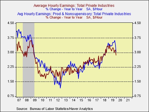
In fact, that’s exactly what we saw.  In November, wage growth for this class of worker rose 3.4%; it fell 40 bps to 3.0% in December.  Thus, the divergence between total private wages and production and non-supervisory worker wages appears to be solely a function of minimum wage laws.  Without additional measures, it seems unlikely that the divergence will continue.

Hours worked:  The growth rate of hours worked by production and non-supervisory workers fell to its lowest level since June 2010.

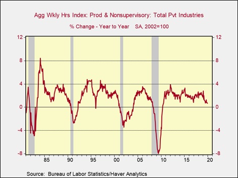
The combination of fewer hours and falling wage growth will tend to further dampen available liquidity for the majority of households.  The weekly hours data isn’t recessionary, but it is headed in that direction.

Out of the workforce:  When the Bureau of Labor Statistics calculates the labor force, it includes those working and looking for work.  Some citizens purposely decide to stay out of the labor force for a myriad of reasons, with age being the most likely.  In other words, as the number of citizens reaching retirement age increases, the percentage of the population that can continue to work will tend to decline as will the potential labor force.  Nevertheless, as the expansion continues, the potential pool of those out of the labor force tends to decrease until a point is reached where it becomes nearly impossible to draw down this group any further.  At that point, wage growth is expected to rise; at the same time, the unemployment rate can’t decline any further because potential new workers become increasingly difficult to find.

The economy may be nearing that point.

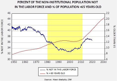
The blue line shows the percentage of those not in the labor force relative to the non-institutional population over the age of 16.  The red line is the percentage of the total U.S. population older than 65, with Census Bureau forecasts.  The area in yellow represents the baby boom generation.  The start of this area is when the last baby boomer turned 16, and the end is when the first baby boomer hit the age of 65.  In the yellow area, the percentage not in the labor force fell and stabilized.  As baby boomers headed into retirement age the percentage not in the labor force began to climb.  However, this percentage has recently stalled, mostly due to the extended economic expansion.  This trend will be difficult to sustain as the 65+ population continues to rise.  Although we are seeing workers delay retirement, the recent trend should reverse over time.  That factor will tend to keep the unemployment rate lower than it has been historically.

What is important about these three trends is that two of them are suggesting some softening in the labor market, whereas the last one might mask that weakness by showing a low unemployment rate.  In other words, older workers, facing a weaker labor market, may simply opt for retirement and leave the labor force entirely.  That will reduce the labor force and keep the unemployment rate low, suggesting the labor market is tighter than it really is.  That factor could increase the potential for a policy error.

View the PDF

by Asset Allocation Committee

In our 2020 Outlook, we discussed three risks to the forecast, with one of them being a “melt-up” or a dramatic rise in stock prices.  One of the key factors that could bolster higher prices for risk assets would be the idea that the FOMC has engineered a soft landing, which is best defined as a tightening cycle that doesn’t result in a recession.

In December 2015, the Fed raised the policy rate by 25 bps, lifting the rate from 0.125% to 0.375%.  The conventional policy models, mostly based on the Taylor Rule, suggested that a series of rate hikes was likely.

This chart shows four variations of the Mankiw Rule, which is different from the Taylor Rule in how it measures slack in the economy.  The former used the unemployment rate, while the latter uses the difference between actual and potential GDP.  We prefer the Mankiw Rule because labor market measures are easily observable, whereas potential GDP is not.  We have created four variations of the Mankiw Rule using various measures of the labor market.  In the chart above, the area highlighted in yellow shows that all the Mankiw variations were suggesting the policy rate was too low and the Fed needed to raise rates aggressively.  The financial markets feared tighter monetary policy but, as the chart shows, after an initial hike the Yellen Fed paused for a year before raising rates again.

Why did this pause occur?  A contributing factor appears to be fragility in the financial markets.

This chart shows the 12-week average of the VIX index of S&P 500 volatility and the fed funds target.  Note that the VIX rose above 20 with the rate hike in December 2015.  It is possible the FOMC worried about triggering broader financial problems by raising rates and thus paused to allow financial markets to “calm down” before raising rates further.

In the recent tightening cycle, the Powell Fed raised rates until the VIX broke 20; soon after, the Fed lowered rates even though the Mankiw Rules would suggest further tightening was in order.  The Fed would be loath for the financial markets to conclude there is a “Fed put,” but, given how sensitive consumption has become to asset values, avoiding a recession may require guiding policy to prevent volatility from rising.

So, if this is what the Fed is doing, what does it mean for equities?  We indexed the S&P 500 to early February 2016, when it became clear that Yellen would keep policy on hold, and January 2019, when Powell signaled at least a pause in tightening.  The idea is that equities should benefit if the Fed avoids a “hard landing.”

The two periods are generally tracking each other; if this pattern continues, the current S&P 500 would end up at 3532.56 by late November.  This analysis is clearly not foolproof as one episode of a soft landing won’t necessarily generate a repeat performance.  Nevertheless, we are tracking relatively closely so further gains in stocks are possible if a recession is avoided.  The trick is avoiding recession; accommodative monetary policy is probably a necessary, but not completely sufficient, condition for avoiding a downturn.

View the PDF

by Asset Allocation Committee

(N.B.  This is our last Asset Allocation Weekly for 2019.  The next edition will be published January 10, 2020.)

Did the Fed engineer a soft landing?  That is the critical question for 2020.  If the Fed, through its rate cuts last year,[1] has rescued the economy, it would be one of the most remarkable episodes of deft central bank practice.

This chart shows fed funds along with recession indicators from the New York and Atlanta Federal Reserve Banks.  The former uses the yield curve in its forecast and the latter uses GDP.  The New York indicator gives a 12-month forward read on the economy.  Since 1970, any reading over 30 for the New York indicator has led to an eventual recession.  Nevertheless, even though its track record is impressive, we like to wait for confirmation from the Atlanta indicator before declaring a downturn.  The chart shows that risks of recession are elevated.

What if recession is avoided?  Because retail money market levels are elevated, we could see a strong rally in equities.

This chart looks at retail money market funds (RMMK) compared to the S&P 500.  When RMMK fell from 2008 into 2011, the equity index more than doubled.  The high level of RMMK may not necessarily all flow to equities, but avoiding recession (and a reduction in trade conflicts) could lead to this liquidity finding its way into asset markets.

In conclusion, the odds of recession are elevated but we don’t see a downturn as imminent.  The FOMC has moved aggressively to cut the policy rate and is at a level we would consider neutral.  If a recession is avoided, risk assets could appreciate significantly in 2020.  However, the risks of a downturn are probably high enough to keep asset prices contained at least for the first few months of the new year.

View the PDF

---

[1] And the expansion of the balance sheet as well.