Asset Allocation Weekly (June 12, 2020)

by Asset Allocation Committee

Although gold is the primary precious metal for investors, platinum, palladium and silver also can fulfill that role.  Complicating matters is that these three metals are dual-use products.  Unlike gold, which has few uses outside of monetary (store of value) purposes and jewelry, these other three have industrial uses as well.  About 55% of silver consumption is in electronics, while 39% is used for jewelry, silverware and monetary reasons.  The remaining 6% of silver consumption is in associated industrial use, including solar panels.  Industry and automotive demand accounts for about 60% of platinum demand, with jewelry absorbing about 30% and investment demand the remainder.  Palladium, which has been in the news lately due to strong price behavior, is mostly used in automobile exhaust systems; nearly 84% of the metal goes into cars, with other industrial uses taking up nearly all the remaining demand.

Thus, unlike gold, the other three precious metals are much more sensitive to industrial activity.  Supply factors are different as well.  Silver is mostly a byproduct of base metal and precious metal mining; only about 28% of silver comes from primary silver mines.  The rest comes from the mining activities of lead, zinc, copper and gold.  Thus, the supply of new silver is affected by the demand for these other metals.  In contrast, platinum and palladium both have limited sources; nearly 75% of new supply of platinum comes from South Africa, whereas 40% of the world’s palladium comes from Russia.

Both gold and silver prices began to rally in the early part of the 2000s after being in the doldrums from the mid-1980s through the 1990s.  High real interest rates depressed demand as policy was designed to contain inflation.  But, around 2003, gold began to rally, and by 2005, silver did as well.  This rally continued into 2011 when silver prices began to fall, and gold followed in 2012.  A stronger dollar weighed on precious metals prices during this period.

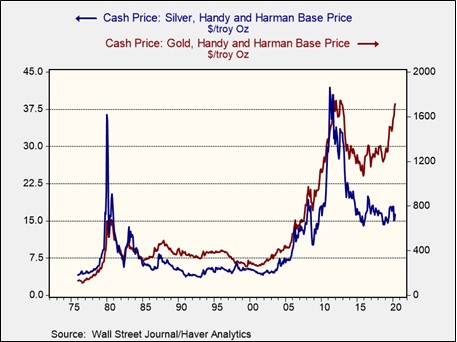
Since 2017, gold prices have clearly outpaced silver, but since August 2018, gold’s outperformance has been substantial.

The gold/silver ratio has been a longstanding way of measuring the relative value of the two metals.

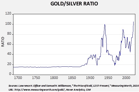
During the gold standard years, many nations conducted a bimetallic system, where gold and silver could be used for money.  The common exchange was 15:1.  The relative scarcity of gold relative to silver led to a widening ratio after the Civil War into WWI.  During WWI, silver prices rose due to expanding industrial activity for the war effort.  The change in the official price of gold by the Roosevelt administration led the ratio to widen out during the 1930s into WWII.  Steadily rising silver prices reduced the ratio to 20:1 by late 1960; in response, the Coinage Act of 1965 dramatically reduced the use of silver in U.S. coins, easing the demand for silver and causing the ratio to rise.

The end of Bretton Woods ended the last remnants of the gold standard, leading to much higher prices for both metals.  Since the mid-1970s, the gold/silver ratio has generally tracked the path of industrial production.  This relationship reflects the industrial demand for silver that doesn’t exist to the same extent for gold.

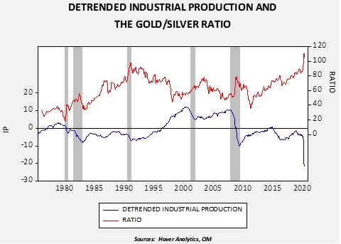
The upper line on the chart shows the monthly gold/silver ratio; the lower line shows detrended U.S. industrial production.  Although the relationship isn’t perfect, in general, stronger industrial production has tended to coincide with a lower ratio, whereas falling and below-trend industrial production benefits gold in the ratio.  The current ratio is near its all-time highs, reflecting (a) generally weak industrial production in the latest business cycle, and (b) the recent collapse in production due to the pandemic shutdowns.

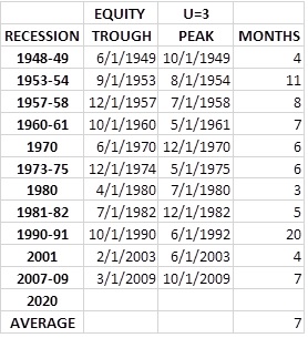
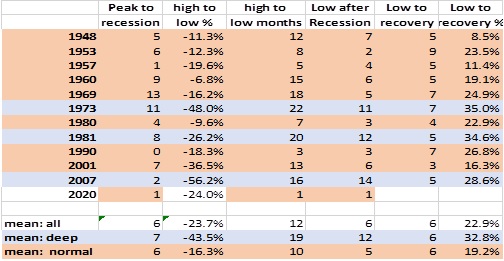
Although there remains a great deal of uncertainty surrounding the path of the recovery, as we detailed recently, the most likely path of this business cycle will be a deep but short recession followed by a lengthy recovery.  If this assessment is correct, industrial activity should rebound in the coming months.  Given the historic level of the gold/silver ratio, coupled with our overall positive position on gold, we believe silver is also attractively valued at current prices if our expectations about the economy are correct.  Therefore, for risk-tolerant investors, silver may be an attractive allocation at this time.

View the PDF

Weekly Energy Update (June 11, 2020)

by Bill O’Grady, Thomas Wash, and Patrick Fearon-Hernandez, CFA

Here is an updated crude oil price chart.  The oil market continues to recover after April’s historic collapse.

(Source: Barchart.com)

Crude oil inventories surprised the markets again, with stockpiles rising 5.7 mb compared to forecasts of a 3.0 mb draw.  The SPR added 2.2 mb this week.

In the details, U.S. crude oil production fell 0.1 mbpd to 11.1 mbpd.  Exports fell 0.4 mbpd, while imports rose 0.7 mbpd.  Refining activity rose 1.3%, above the 0.6% rise forecast.  As we have seen in recent weeks, the level of unaccounted-for crude oil remains elevated.

Unaccounted-for crude oil is a balancing item in the weekly energy balance sheet.  To make the data balance, this line item is a plug figure, but that doesn’t mean it doesn’t matter.  This week’s number is -0.9 mbpd.  For the fifth week in a row, this number is running nearly 1.0 mbpd.  The 12-week average has now gone negative for the first time since October 2017.  It may mean that in the scramble for finding storage, some oil is being inventoried outside the survey system.  This week, some 7.0 mb of crude oil went into storage somewhere, just not where it can be recorded.  Or, production is falling much faster than the DOE estimates are capturing so there aren’t any missing barrels; simply put, production is cratering.  The DOE did indicate it had made modest downward revisions to production, but we are increasingly leaning toward the idea that production is falling rapidly, much faster than the DOE is able to record.

(Sources: DOE, CIM)

The above chart shows the annual seasonal pattern for crude oil inventories.  This week’s data showed a rise in crude oil stockpiles.  We are getting close to the beginning of the seasonal draw for crude oil.  If inventories don’t decline in the coming weeks, oil prices would be vulnerable to a correction.

Based on our oil inventory/price model, fair value is $27.65; using the euro/price model, fair value is $51.76.  The combined model, a broader analysis of the oil price, generates a fair value of $39.87.  We are starting to see a wide divergence between the EUR and oil inventory models.  The weakness we are seeing in the dollar, which we believe may have “legs,” is bullish for crude oil and may overcome the bearish oil inventory overhang.

Although gasoline consumption is improving, the distillate market is becoming a worry.

Distillates are the fuels of commerce; trucks, trains, planes and ships run on this fuel.  The weakness in consumption suggests that wholesale activity is probably slumping.  Perhaps the restocking of inventory that occurred after the initial decline is waning and the subsequent pickup is soft.  But the weakness here will tend to keep refinery activity slow and may cap the recent recovery in oil prices.

Although there are anecdotal reports that shale production may be restarting, history shows that there is about a five-month lag between prices and drilling activity.  That would suggest production overall will likely remain depressed well into Q4.

This chart shows oil and gas drilling activity from the industrial production data; in general, oil prices lead this measure by about five months.  If this pattern is maintained (and there is little reason to see why it won’t), we probably won’t see a recovery in drilling until much later this year, which is bullish for crude oil prices.

In politics and geopolitics this week, Iran has built a likeness of an aircraft carrier to allow its naval forces to train against.  Iran did something similar in 2015.  As U.S. forces leave Iraq, Islamic State activities are returning.  Although they are not in oil-producing areas, a return of IS would be bad news for Iraq.  We continue to monitor developments in Libya; currently, Khalifa Hifter’s forces have been reeling in the face of Islamic-leaning groups in western Libya who have been supported by Turkey.  We are seeing intermittent oil output disruptions.  China has been showing interest in increasing its influence in the Middle East.  Given China’s oil dependence, increasing its activity in the region makes sense, especially as the U.S. reduces its regional footprint.  However, we are surprised at Beijing’s increasing interest in Syria, which is a very small oil producer.  It will be interesting to see how Putin reacts to such behavior.  Although elements within the Democratic Party have pushed to severely restrict oil and gas drilling for environmental reasons, minority groups within the party are pushing for jobs in the sector.

View the PDF

Weekly Geopolitical Report – The Geopolitics of the 2020 Election: Part III (June 8, 2020)

by Bill O’Grady | PDF

In this five-part series on the geopolitics of the 2020 election, we have divided the reports into nine sections. Last week, in Part II, we discussed the second and third sections, understanding the electorate and party coalitions.  In this report, we continue our coverage with the fourth and fifth sections, the incidence of the establishment coalition and the impact of social media.

Read the full report

Asset Allocation Weekly (June 5, 2020)

by Asset Allocation Committee

Last week, we discussed how equity markets, because of their anticipatory nature, tend to bottom in advance of the end of recessions.  Assuming that condition continues, if our expectations for a short recession (but probably a long recovery) are correct, it would make sense that the equity market would have already bottomed.  That historical pattern, coupled with extraordinarily supportive monetary policy, is supporting equity values.

The view of the economy for most Americans is the job market.  In general, the common belief is that a good economy is one with a good job market.  Economists tend to take a broader view and assume that the economy is more than just jobs.  And so, when overall economic activity recovers, recessions are declared over.  However, there are numerous cases where the economy and equity markets are doing fine, while the labor markets are still sluggish.

This chart shows the S&P 500 with the unemployment rate.  We have placed black vertical lines at the trough of the equity index (using S&P 500 monthly averages) and a red line at the peak of unemployment.  Here is a table of the results.

This table shows that equities trough about seven months before the peak of the unemployment rate.  Thus, if the unemployment rate has peaked the turn in equity markets seen in recent weeks would be consistent with that pattern.  The full recovery in the labor markets will take much longer, but we do expect labor market conditions will steadily improve.

View the PDF

Weekly Energy Update (June 4, 2020)

by Bill O’Grady, Thomas Wash, and Patrick Fearon-Hernandez, CFA

Here is an updated crude oil price chart.  The oil market continues to recover after April’s historic collapse.

(Source: Barchart.com)

Crude oil inventories surprised the markets for the fourth straight week with stockpiles falling 2.1 mb compared to forecasts of a 3.0 mb build.

In the details, U.S. crude oil production fell 0.2 mbpd to 11.2 mbpd.  Exports fell 0.4 mbpd, while imports declined 1.0 mbpd.  Refining activity rose 0.5%, a bit below expectations.  As we saw last week, there was another jump in unaccounted-for crude oil.

Unaccounted-for crude oil is a balancing item in the weekly energy balance sheet.  To make the data balance, this line item is a plug figure, but that doesn’t mean it doesn’t matter.  This week’s number of -1.01 mbpd is the largest negative number on record.  For the fourth week in a row, this number is running nearly 1.0 mbpd.  The 12-week average is on the verge of going negative for the first time since October 2017.  It may mean that in the scramble for finding storage, some oil is being inventoried outside the survey system.  This week, the SPR took 4.0 mb, but that doesn’t resolve the unaccounted-for crude issue.  This week, some 7.0 mb of crude oil went into storage somewhere, just not where it can be recorded.  Or, production is falling much faster than the DOE estimates are capturing so there aren’t any missing barrels; simply put, production is cratering.  We still don’t know which thesis is correct.  However, given the persistence in the unaccounted number, it is looking increasingly likely the DOE is overestimating production.

(Sources: DOE, CIM)

The above chart shows the annual seasonal pattern for crude oil inventories.  This week’s data showed a modest decline in crude oil stockpiles.  We are getting close to the beginning of the seasonal draw for crude oil.  If inventories don’t decline in the coming weeks, oil prices would be vulnerable to a correction.

Based on our oil inventory/price model, fair value is $29.12; using the euro/price model, fair value is $45.01.  The combined model, a broader analysis of the oil price, generates a fair value of $36.57.  It does appear that the worries over storage capacity have been resolved, so the model is more reliable.  We have been seeing a steady drop in the dollar recently.  The Eurozone is considering a mutualized debt instrument to pay for COVID-19 costs.  It is possible the Eurozone may use this event to create a permanent mutualized Eurobond which would make the EUR an attractive alternative to the dollar for reserve purposes.  A weaker dollar would be bullish for oil prices.

In energy news, the Kingdom of Saudi Arabia (KSA) moved liquidity from its foreign reserves to its sovereign wealth fund.  The fund has been aggressively buying assets overseas, viewing the current weakness caused by the virus as a buying opportunity.  Foreign reserves act as a buffer to low oil prices and so a decline in reserves may force additional austerity measures on the populous.

This chart shows the KSA’s foreign reserves and Brent oil prices.  Lower oil prices tend to reduce reserve levels with a lag.  Thus, the decision to shift funds to the soverign wealth fund may reflect the idea that oil prices will rebound quickly.

In OPEC news, there are doubts the cartel will hold an early meeting.  This news eased prices modestly.  We expect the cartel and Russia will maintain production cuts for at least another month.  Venezuela says it will increase gasoline prices, a risky move for a nation with heavily subsidized petrol.

VP Biden is considering new climate proposals; if elected, these measures may reduce oil production.  The Trump administration has reduced states’ ability to regulate energy companies; that may reverse under a Biden government.

This week, we want to discuss the natural gas market.  May is the “shoulder month” for demand.  As summer unfolds, demand for electricity tends to rise and, if temperatures are high enough, helps boost natural gas prices.  First, here is the supply/demand balance.

Currently, there is a rather wide supply imbalance, with supply outpacing consumption.  Under these conditions, inventories tend to accumulate.  The chart below shows seasonally adjusted working natural gas storage.  Inventory levels are well above normal as we head into summer.

One bright spot is that the supply/consumption balance is showing some improvement.  If we see hot weather in the coming weeks, it should allow the inventory overhang to dissipate and support prices.  Another bullish factor is that falling oil production will reduce associated natural gas production, which should help narrow the inventory overhang.  However, any bullish scenario rests on an unusually hot summer.  The current summer forecast is leaning hot, so there is the potential for a price recovery in the coming weeks.

View the PDF

Weekly Geopolitical Report – The Geopolitics of the 2020 Election: Part II (June 1, 2020)

by Bill O’Grady | PDF

In this five-part series on the geopolitics of the 2020 election, we have broken the reports into nine sections. In Part I, we covered the basics of public finance.  This week, we will cover the second and third sections, understanding the electorate and party coalitions.

Understanding the Electorate
Understanding the electorate is about divining the psychological and economic interests of voters.  In this section, we describe how we examine the voting public.

There is a distinction between class and identity.  Identity is complicated.  All of us belong to various groups based upon our gender, race, religion, age, geographic location, education, etc.  The interlacing of these various memberships is known as intersectionality.  Although the term is often applied to those who face discrimination, in general, this term captures the various “tribal” groups to which we find ourselves belonging.  Thus, a white, gay, Catholic with a graduate degree may have something in common with a Hispanic, straight, Catholic with a high school diploma through their religious affiliation.  However, it is unlikely the commonality would be very strong.  In general, the greater the identity overlap a person has with others the higher the probability they will vote for or favor candidates of a similar persuasion.  At the same time, each person tends to “rank order” their identities; some put a much higher rank on race relative to religion, for example.  Or, their geographic location is the most important identity classification.

Class is rather straightforward, determined by the decile in which one’s income and wealth falls.  This breakdown isn’t perfect, however, as the class interests between two people with equal income can differ.  For example, if two middle managers at different firms make the same income, but one manager’s firm benefits from free trade and the other does not, they may favor different economic policies.  But, in general, policies favored by class tend to be uniform.  For example, the wealthy tend to have similar positions on taxes, while the less affluent tend to think very highly of Social Security.

We define a group as the cross-section of identity and class.  A group is a set of like-minded people who tend to support similar political, economic and social positions.

To describe the interplay between identity and class, we have borrowed this grid from Peter Zeihan.

Read the full report

Asset Allocation Weekly (May 29, 2020)

by Asset Allocation Committee

The recent strong rally in equities has befuddled investors—how can equities rally with such vigor when the economy is historically weak?  We suspect there are two reasons for this recovery:

  1. Although the drop in economic activity is deep, it will likely be short.
  2. Supportive monetary policy is a powerful elixir for equities.

Equity markets are forward-looking; investors put their money to work on expectations of future economic conditions and earnings, not based on what is occurring today.  The current downturn is historic.  The decline in the economy has been very fast and deep, but it will likely be short.  In fact, the recovery should begin by midsummer at the latest.  We use these words to mean something specific.

This chart shows a stylized path of the business cycle.  Orange represents expansion, when the economy is making new peaks in an indicator.  This can be GDP, industrial production, coincident indicators, etc.  Blue is recession and is measured from peak to trough.  Green is recovery, which lasts from trough until a new peak occurs.  Finally, once a new peak is made, a new expansion is underway.

We expect this recession to end quickly because the trough will probably occur in Q2.  However, the recovery will be long and likely dictated by the path of the virus.  We currently estimate the new expansion will start in H2 2021.

(Data source: Haver Analytics)

This table shows the declines in the S&P 500 for the postwar recessions.  On average, equities tend to peak about six months before the onset of the economic downturn, while the low occurs about six months after the peak in economic activity.  From the market low to recovery, the S&P 500 usually rebounds by about 20%.  But, notice from deep recessions that the rebound from the low is about 33%.  The rebound we have witnessed thus far is in line with a deep downturn, but it appears unusual due to the compressed nature of the current recession.

Also noted above are the aggressive actions taken by the FOMC.  Below is a chart that will be familiar to regular readers.

From early 2009 until November 2016, the path of the S&P 500 closely matched the Fed’s balance sheet.  There was always concern that the relation was a spurious correlation, and the behavior from December 2016 into August 2019 suggested it was.  However, it is important to note that equities were buoyed by expectations of a massive corporate tax cut.  Taking the balance sheet and incorporating the tax cut gives us a model that offers some insight into the impact of current monetary policy.

Fair value is derived from smoothing the higher marginal rate of the corporate tax and the balance sheet.  Adding the impact of the tax cut accounts for some of the rally in equities.  The sharp rise in the fair value in recent months reflects the massive expansion of the balance sheet.

This is not our forecast for the S&P 500, but it does offer some insight into how powerful the Fed’s actions have been.  We doubt the equity index will track this model due to the level of uncertainty surrounding the path of the economy.  Nevertheless, a projected short, sharp downturn coupled with the most rapid increase in the balance sheet since WWII have created strong support for equities that will likely prevent significant corrections, barring a major policy error or an unexpected negative turn in the toxicity of the virus.

View the PDF

Weekly Energy Update (May 29, 2020)

by Bill O’Grady, Thomas Wash, and Patrick Fearon-Hernandez, CFA

Due to the Memorial Day holiday, the DOE data was delayed until yesterday.  Thus, our report was delayed as well.  Here is an updated crude oil price chart.  The oil market continues to recover after April’s historic collapse.

(Source: Barchart.com)

Crude oil inventories surprised the markets for the third straight week but this time by rising 7.9 mb compared to forecasts of a 2.5 mb draw.

In the details, U.S. crude oil production fell 0.1 mbpd to 11.4 mbpd.  Exports were unchanged, while imports rose 2.0 mbpd.  Refining activity rose 1.9%, above expectations.  As we saw last week, there was another jump in unaccounted-for crude oil.

Unaccounted-for crude oil is a balancing item in the weekly energy balance sheet.  To make the data balance, this line item is a plug figure, but that doesn’t mean it doesn’t matter.  This week’s number of -999 kbpd is the largest negative number on record.  For the third week in a row, this number is running nearly 1.0 mbpd.  It may mean that in the scramble for finding storage, some oil is being inventoried outside the survey system.  In other words, over the week, some 6.9 mb of crude oil went into storage somewhere, just not where it can be recorded.  Or, production is falling much faster than the DOE estimates are capturing so there aren’t any missing barrels; simply put, production is cratering.  We still don’t know which thesis is correct.  Given that imports rose this week, some of the unaccounted-for crude oil may be in storage floating on the ocean and prices have reached a point where some of it is coming ashore.  Nevertheless, it is still quite possible that production is falling faster than estimated.[1]  The second factor is that the SPR rose 2.1 mb as some of the oil went into the strategic reserve.

(Sources: DOE, CIM)

The above chart shows the annual seasonal pattern for crude oil inventories.  This week’s data showed a rebound in crude oil stockpiles.  We are getting close to the beginning of the seasonal draw for crude oil.  If inventories don’t decline in the coming weeks, oil prices would be vulnerable to a correction.

Based on our oil inventory/price model, fair value is $28.43; using the euro/price model, fair value is $44.74.  The combined model, a broader analysis of the oil price, generates a fair value of $36.10.  As we have noted recently, the model output is less relevant as there is a non-linearity tied to the loss of storage capacity that cannot be fully captured with these models.  At the same time, if storage remains available, the models would suggest further upside for oil prices.

Although consumption remains depressed, there are reports that driving is starting to recover as lockdown rules ease.  The gasoline supplied data on the chart below also continues to show improvement.  Some data tracking does suggest an upswing in driving activity.

Another way of looking at gasoline is comparing inventories to consumption and calculating how many days of inventory are available at current consumption rates.

The current level is about 10 days above average.  An interesting sidelight is that the drop in gasoline demand has led to a drop in ethanol demand as well.  We get carbon dioxide from processing corn for ethanol which is sold to make fizzy drinks, dry ice, etc.  The price of CO2 is rising.

In market news, the IEA warned that shale investment would likely halve in 2020.  Venezuela received a shipment of gasoline from Iran.  Both nations violated U.S. sanctions; so far, there hasn’t been a notable response from the U.S.

View the PDF


[1] The weekly production numbers are estimates.  The official data comes with a two-month lag.  The DOE data for April indicates that production was 12.7 mbpd…but even that was an estimate.