

Asset Allocation Weekly (May 15, 2020)
by Asset Allocation Committee
As the Federal Reserve expands its balance sheet and the federal deficit balloons, there is a legitimate concern about the potential for inflation. In this week’s report, we will examine inflation from a theoretical perspective.
There are two simple tools we use to discuss inflation, the equation of exchange and the intersection of aggregate supply and demand. To start, this is the equation of exchange:
MV=PQ
M is the money supply and V represents the speed at which it is spent; on the other side of the equation is P, the price level, and Q, output. In the calculation of the variables, the right side of the equation is nominal GDP and M is one of the various formulations of the money supply. However, the power of the equation, in our opinion, comes from what the variables represent. For example, Q is best thought of as the productive capacity of the economy, the ability of an economy to procure goods and services. It would include not just actual production, but also excess capacity. And V isn’t just a residual; it can tell us the effectiveness of money policy.
The classical economists assumed that V and Q were fixed; V represented the institutional structure of money demand and thus only changed when spending and income patterns were adjusted. Since prices were flexible, Q was always at full employment and thus didn’t change. If these assumptions were true, any increase in M would lead to a proportional rise in P. However, it turns out neither V nor Q were fixed; in some periods, increasing M led to higher price levels, but in others, it did not.
In the last episode of the Federal Reserve balance sheet expansion, velocity fell, leaving prices and quantity mostly unchanged.
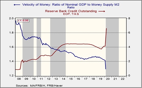
This chart shows calculated velocity and the Fed’s balance sheet. The gray shaded areas indicate periods of official QE. Note that there is a strong inverse correlation between velocity and the balance sheet expansion, suggesting that households and businesses are not demanding the funds being provided to the banking system. Thus, the inflationary impact of expansionary monetary policy has been reduced. Given current risks in the economy and markets, we would expect the current balance sheet expansion to lead to a similar result in the short run—another decline in velocity.
The second tool is aggregate supply and aggregate demand. Although neither of these can be calculated with any degree of confidence, we can use the tools for illustration.
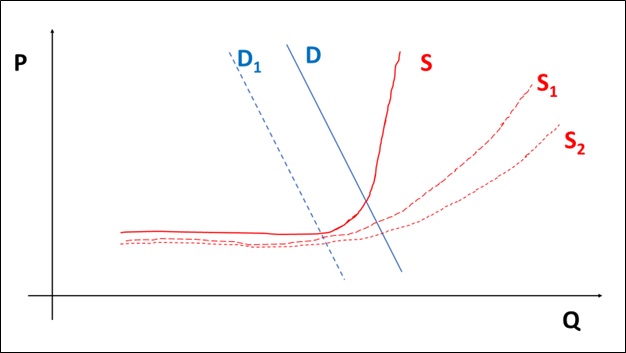
The key point to this schematic lies in the supply curves, labeled S, S1 and S2. The latter is what we believe is our current supply curve; demand has shifted from D to D1. One of the consequences of COVID-19 is that we expect the trend toward deglobalization to accelerate, which would likely mean a shift in the supply curve from S2 to S1. As deglobalization is eventually tied to reregulation of the economy, we will shift to S. Of course, the key to rising prices will be the path of demand. The longer it takes for demand to recover, the less likely it is that inflation will return with any significance. However, when demand returns, we will likely see upward price pressures; if rising demand coincides with the eventual shift to the terminal supply curve S, the markets could be in for a notable inflation surprise. We don’t expect this terminal shift to occur in the next three years, but it is highly likely in the latter half of the decade.
Tying this back to the equation of exchange, the supply curves above are represented by Q. So, as supply becomes increasingly constrained, velocity will need to fall further in order for prices to remain steady as the money supply rises. If inflation expectations change, it would be reasonable to expect velocity to increase, which would tend to lead to higher inflation. The key points from this analysis are that (a) Fed policy actions, in isolation, are not necessarily inflationary, and (b) constraining supply, which is an element of deglobalization, could lead to higher price levels once demand recovers.